Adaptive-optical 3D microscopy for microfluidic multiphase flows

Fluid flows influence the efficiency and yield in many technical processes significantly and therefore offer a large potential for optimisation. For instance, the dynamics of liquid films and droplets on surfaces is of high importance in many manufacturing processes, such as electronic devices manufacturing¹ or coating applications². Thin film flows are used to create functional surfaces or barriers, which need to fulfil certain criteria like homogeneous thickness, controlled deposit of suspended particles, etc. Variations in final film thickness are often caused by uneven delivery of liquid during the manufacturing process or the natural wave-formation of film flows in combination with the time scales of the levelling of the film^3,4. In manufacturing processes (uncontrolled) waviness of the liquid film as well as curved shapes like e g. beads will lead to for instance coating defects.

Another example of curved liquid shapes in manufacturing processes is the use of drops, e. g. in ink-jet-like drop-on-demand deposition of active pharmaceutical ingredients⁵ or liquid metal jet printing, as a nascent additive manufacturing technology that has the potential to fabricate metallic components⁶. Moreover, droplets play an important role in the water management of Proton Exchange Membrane Fuel Cells (PEMFCs)⁷. In PEMFCs hydrogen and oxygen react to form water. However, a too high amount of liquid water, usually in the form of droplets, blocks the transport of oxygen to the catalyst⁸ which results in a significant voltage drop and reduced efficiency.

Many of these applications would profit from better models for predicting the inner fluid motion of droplets⁹ and film flows. However, due to difficulties in simulation and measurement of multiphase flows, predicting the behaviour of films and drops is still challenging and experimentalists and modellers work on that alike for decades^10,11. The challenge to simulate the aeroelastic behaviour of the liquid-gas phase boundary is one of the largest hurdles for achieving precise results¹². Similarly, measurements of the micrometer-scale flow field¹³ are difficult because in many cases the only optical access is the fluctuating liquid-gas boundary. Usually, imaging-based techniques are employed because of their high spatial and temporal resolution. Flow measurements are performed by adding micrometer-size particles to the fluid that are imaged, localized and tracked to reveal the fluid motion. In the case of liquid-gas boundaries, dynamical aberrations are introduced by the time-dependent refraction at the interface which results in blurred and dislocated particle images and hence in an increased measurement uncertainty^14-16. In principle, the opaque substrate can be replaced by a transparent surface to allow access. However, this substantially changes the flow¹⁷ and is not always possible (e g. bubbles, porous substrates). Hence, measurements of multiphase flows with low optical accessibility are challenging up to now.

In this manuscript, we present high-speed 3D localisation microscopy with a real-time adaptive optics correction as a solution for this challenge. A custom-manufactured phase mask combined with an ultra-fast camera enables monocular imaging and tracking of fluorescence particles with frame rates of 800 Hz. The adaptive optics system consists of a deformable mirror with a settling time of 0.8ms which is controlled by a custom-developed low-latency electronic control unit. Wavefront sensing is implemented with a custom-developed Hartmann-Shack sensor that offers a direct interface to the electronic control unit so that control rates up to 3600 Hz are possible. Exemplarily, we apply this approach to droplets on a Gas Diffusion Layer (GDL), since this is a typical case which does not allow an optical access through the substrate, to correct a systematic error that affects the periodic flow field. By doing so, we demonstrate for the first time that adaptive optics can decrease the measurement uncertainty of a two phase flow in which the phase boundary motion and the inner flow are coupled. Our results show a potential for achieving a better understanding of dynamic microscopic flow fields coupled with a phase boundary, which can for instance facilitate the optimisation of droplet removal in fuel cells.

Adaptive optics has been employed for many different applications, as for instance correction of atmospherical^18,19 or oceanic²⁰ turbulence, control of the intensity distribution in laser processing²¹ and correction of thermally-induced aberrations²². In microscopy, it is well-known particularly for imaging deep within tissue of biological samples²³. Another application is the microscopic imaging and tracking of particles for flow field reconstruction through a fluctuating water-air interface. Both cases have in common that refractive index inhomogeneities between the object to be imaged and the microscope objective introduce aberrations (Fig. 1). In the following, we discuss the consequences that arise for our special case in terms of system engineering.

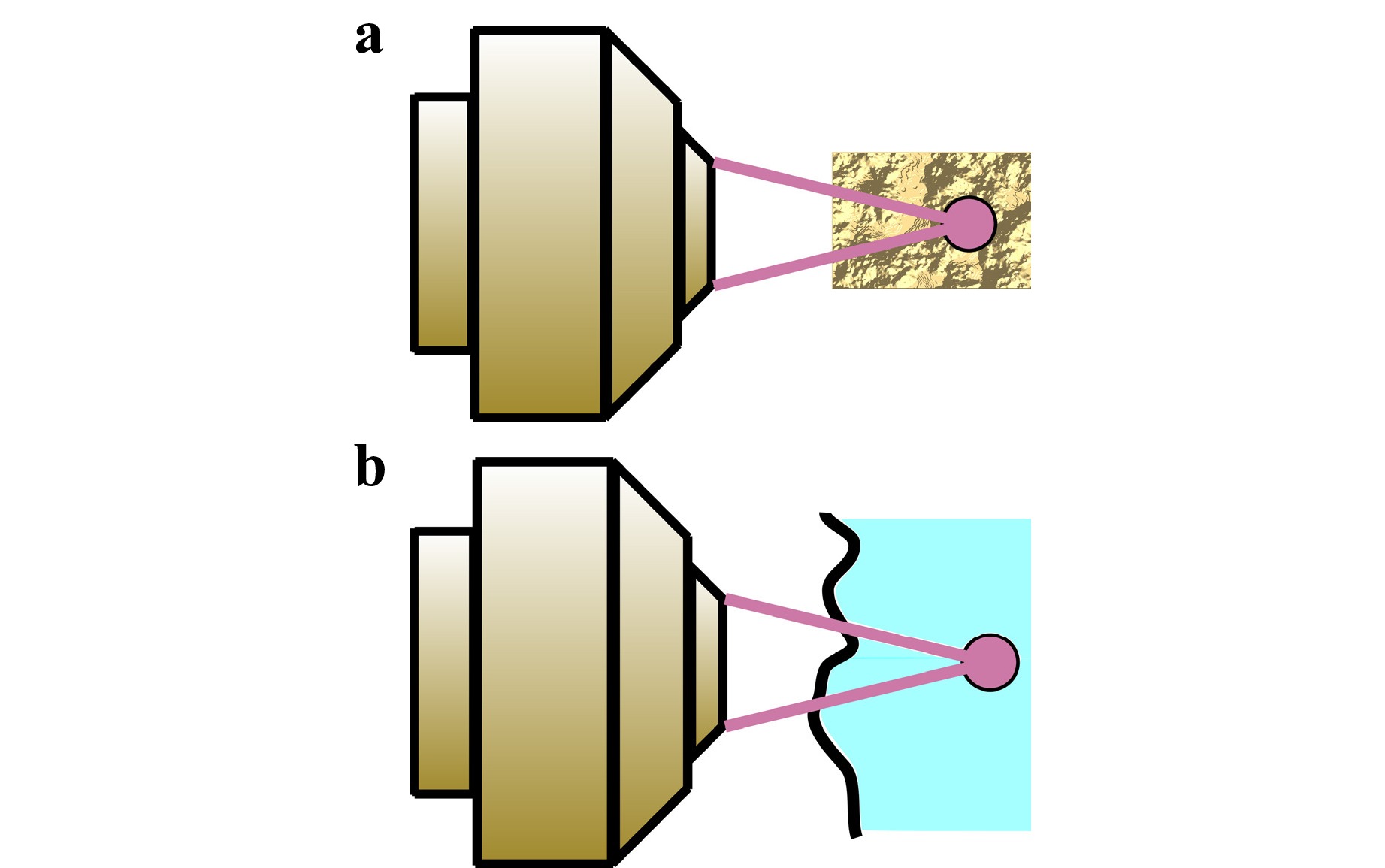
Fig. 1  Comparison of microscopical imaging of fluorescence markers through a biological tissue and b a temporally fluctuating water-air interface. In both cases, the sample induces aberrations that decrease the imaging quality. A difference is that the aberrating layer is three-dimensional in a (similar to atmospheric turbulence) and quasi-planar in b.

1. Aberrations introduced by tissue have their origin in the spatially-varying refractive index of a three-dimensional volume (as well as scattering), whereas the waves on a water-air interface introduce aberrations due to refraction at a relatively thin (quasi-planar) layer. As a consequence, the size of the corrected Field of View (FOV) can be increased by placing the adaptive-optical component (e. g. deformable mirror) in a conjugate plane to the aberrating layer (water-air interface)^24,25, instead of the pupil plane, as it is the case for most adaptive-optical microscopes. Furthermore, the computation of the correcting set value (for the deformable mirror) can be realised without iterative control techniques based on a sharpness metric, if the shape of the water surface is known.

2. In contrast to the usually temporally quasistatic aberrations induced by tissue, liquid-gas interfaces typically exhibit frequencies between roughly 5Hz and several hundred Hertz. Therefore, the bandwidth of the closed-loop disturbance rejection needs to be significantly higher. Besides that, a software based correction similar to lucky imaging in astronomy²⁶ is not straightforward to implement because the dynamical aberrations and the true flow field change with approximately the same time constants.

Fig. 2 illustrates the basic principle of the optical setup. As usual in fluorescence microscopy with epi-illumination, excitation light is coupled into the system with a beam splitter (probe beam in Fig. 2). The laser beam is collimated by the tube lens and the objective, so that the measurement object is illuminated volumetrically. Subsequently, the fluorescent light of the particles is imaged to the camera, which records the particle distribution for tracking.

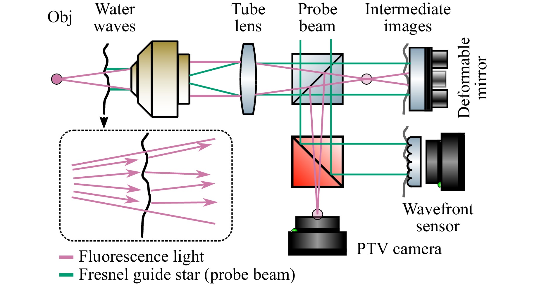
Fig. 2  Simplified overview of optical setup. The rays of the fluorescence particle are refracted by the fluctuating water-air interface. Because this aberrating layer can be considered planar, the correction performance can be increased by placing the deformable mirror in a conjugate plane to the water-air interface. The height profile of the water surface is sampled with a probe beam (green), which we term Fresnel Guide Star (FGS), and a wavefront sensor. The probe beam (FGS) is coupled into the system via a beam splitter and its reflex at the water-air interface is imaged to the deformable mirror and the wavefront sensor. For the sake of simplicity, the 3D localisation microscope is illustrated here as 2D microscope.

The water waves introduce dynamical aberrations to the fluorescence microscopy image, which results in distorted fluctuating particle images. In order to correct for this disturbance, the excitation light beam not only serves for fluorescence excitation, but instead it is also used for measuring the water-air interface. Although most of this light transmits this interface (and excites fluorescent particles), approximately $ ((n_{\text{F}} - n_{\text{A}})/(n_{\text{F}} + n_{\text{A}}))^2 = 2{\text{%}} $ of it is reflected according to the Fresnel equations at perpendicular incidence, where $ n_{\text{F}} = 1.33 $ and $ n_{\text{A}} = 1.0 $ are the refractive indices of water and air, respectively. A 4f-system images the reflected light rays from the water surface to a Hartmann-Shack wavefront sensor, which is possible because imaging with 4f systems conserves the ray angles except for a scaling factor. We refer to the light beam used for probing the water surface as Fresnel Guide Star (FGS) because of its similarities to the Laser Guide Stars (LGSs) in astronomy²⁷ to determine the occuring aberrations. The knowledge about the shape of the water surface then makes it possible to estimate its influence on the refracted fluorescence light rays, so that this effect can be corrected in a closed-loop with a deformable mirror.

Fig. 3 shows a detailed sketch of the optical setup, which also includes information about the three-dimensional localisation microscope. In the following, the operating principle of the adaptive optics system and the 3D microscope will be presented separately. Firstly, the optical setup (with focus on the individual components) as well as the closed-loop control of the adaptive optics system is discussed. This is followed by the description of the three-dimensional microscopy system based on the Double-Helix Point Spread Function (DH-PSF).

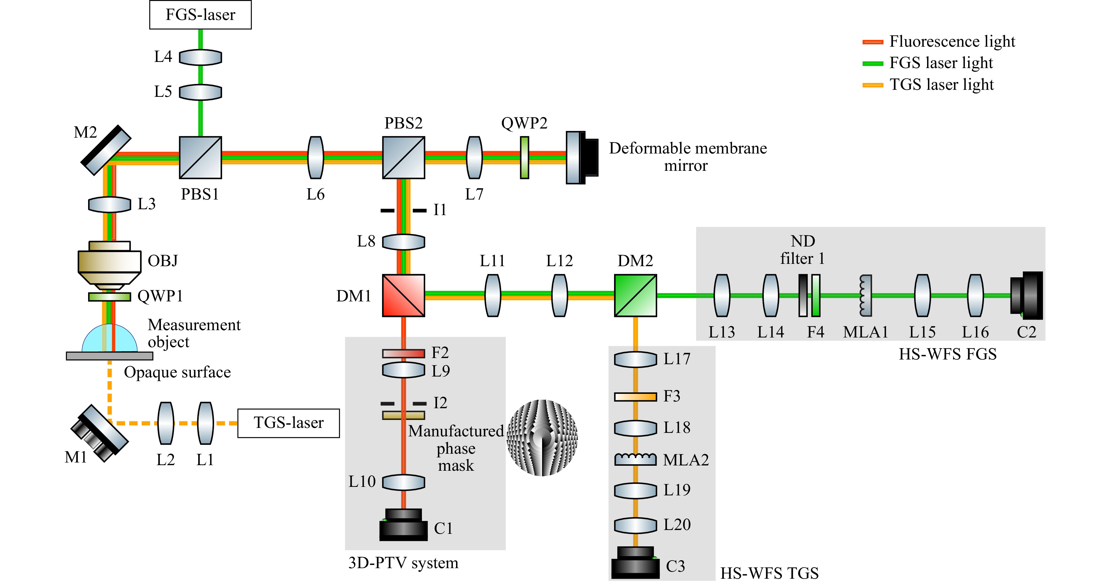
Fig. 3  Simplified illustration of the optical setup with the spiral phase mask implemented at the lithographically manufactured phase mask and the aberration correction with the deformable mirror. M: Mirror, L: Achromatic Doublet Lens, OBJ: Objective, I: Iris Diaphragm, C: Camera Sensor, F: Spectral Filter, MLA: Microlens Array, PBS: Polarising Beam Splitter, DM: Dichroic Mirror, TGS: Transmitting Guide Star, HS-WFS: Hartmann-Shack Wavefront Sensor, FGS-Laser: 532 nm - cw, TGS-Laser: 561 nm - cw.

A 532-nm laser beam (RLTMGL-532-1W-3 from Roithner Lasertechnik GmbH) for exciting the fluorescent particles and measurement of the water surface is coupled into the system with the beamsplitter PBS1, from where it propagates to the air-water interface. The reflected light rays of the FGS are imaged to the deformable mirror with the objective (TL10X-2P from Thorlabs, 10x, NA = 0.5), the tube lens L3 and a subsequent 4f system (L6-L7). The comparatively large working distance of 7.77 mm of the objective at a relatively large numerical aperture of 0.5 makes it a good choice for microfluidic measurements with high light efficiency, which is explained in more detail in the section 3D Microscopy. The reflected light changes its polarisation state due to the quarter-wave plate QWP1 and therefore it passes PBS1. The deformable mirror (DM69 from Alpao in France, 69 actuators, diameter of 10.5 mm) offers a fast settling time (0.8 ms) and thus enables the correction of dynamical aberrations with high bandwidth. In the next step, the intermediate image of the water interface at the deformable mirror is imaged to the wavefront sensor with three 4f systems (L7-L8, L11-L12, L13-L14). By using the achromatic quarter-wave plate QWP2, almost all of the FGS light reflected at the water surface is guided towards the deformable mirror and afterwards to the wavefront sensor. Wavefront sensing is implemented with a Hartmann-Shack sensor that consists of the microlens array MLA1 (APO-Q-P250-AR0.386 from Advanced Microoptic Systems GmbH, Germany) whose focal plane is imaged to the high-speed camera C2 with lenses L15-L16 so that about 5 × 5 focal spots are available. The high-speed camera is custom-developed (sensor: LUPA3000, subset of 256 × 256 px in the center is used, max. 10,704 fps) and directly connected to the Field Programmable System-on-a-chip (FPSoC) so that the delay due to signal processing is minimised¹⁴. The wavefront of the static water-air interface is measured before the experiment as a calibration value for zero aberrations. In order to verify and calibrate the aberration measurement via FGS experimentally, a laser beam which we term Transmission Guide Star (TGS) is implemented below the measurement object (Fig. 3). Naturally, this guide star is not enabled for the measurement in droplets on opaque surfaces.

For ensuring stability and good disturbance rejection of the closed-loop system, the control rate must be sufficiently high. Although this value can depend significantly on the underlying system dynamics and the controller type, a frequently applied rule of thumb is that the control rate should be at least 10 times the bandwidth of the controlled system²⁸ which is about 1.5kHz for frequencies up to 150 Hz²⁹. Therefore, the image processing algorithms for the Hartmann-Shack sensor as well as some parts of the control algorithm are implemented on a custom developed embedded system. It is based on the FPSoC Zynq-7100 which comprises two processors and one Field Programmable Gate Array (FPGA) which makes it possible to achieve control cycles up to 3600 Hz and disturbance rejection up to 150 Hz. Details about it can be found in¹⁴. The controlled system is essentially a multiple-input and multiple-output (MIMO) system with 69 inputs (number of mirror actuators) and $ 2 N_B $ outputs, where $ N_B $ is the number of focal points at the FGS Hartmann-Shack sensor. The static relationship between input and output is assumed to be linear according to³⁰

where $ y_B \in \mathbb{R}^{2 N_B} $ is the system output and $ u_a \in \mathbb{R}^{69} $ the input. However, the matrix $ B \in \mathbb{R}^{2 N_Bx69} $ is not calculated or measured directly. Instead, a virtual input $ u_z \in \mathbb{R}^{N_z} $ with $ u_a = C \cdot u_z $ is created, where $ N_z $ denotes the number of controlled Zernike polynomials. The column $ i $ of $ C \in \mathbb{R}^{69xN_z} $ contains the actuator values for displaying the Zernike polynomial $ i $ on the deformable mirror. After that, relationship 1 can be written as $ y_B = M \cdot u_z $, where the static gain matrix $ M \in \mathbb{R}^{2 N_BxN_z} $ can be identified easily experimentally by measuring $ y_B $ for different $ u_z $. In order to approximately decouple the MIMO system into $ N_z $ single-input-single-output (SISO) systems, the correcting set value for the FGS is identified by the Moore-Penrose inverse as

However, it must be considered that we want to correct the aberrations of the refracted particle light and not the wavefront of the distorted FGS. Therefore, the correcting set value $ \hat{u}_{z,T} $ for the refracted light needs to be estimated from $ \hat{u}_{z} $ of equation 2, which is described in section 3. After that, for each row of $ \hat{u}_{z,T} $ a SISO Proportional–Integral–Derivative (PID) controller controls the corresponding Zernike polynomial shape on the mirror.

Three-dimensional particle tracking with only one optical access is realised using monocular 3D microscopy. Although many different types exist³¹, the technique based on the DH-PSF was chosen due to its success in biology^32-34 and its relative simplicity. The basic idea is to modify the point spread function of the system so that the three-dimensional position of a point emitter can be retrieved precisely from its image intensity pattern.

The key components of the 3D localisation microscope are the objective, the phase mask and the camera. The super-apochromatic objective (TL10X-2P from Thorlabs) offers a reasonable numerical aperture of 0.5 for a large FOV of 2.2 mm as well as a comparatively large working distance of 7.77 mm, which makes it a good choice for fast fluorescence imaging of millimeter-scale objects. The spatial modulation in the pupil plane is achieved by employing a lithographically custom-manufactured phase mask. Details about it and a comparison with a liquid-crystal based Spatial Light Modulator (SLM) can be found in the following section. The implemented high-speed camera C1 (Phantom v1610) offers a high frame rate of up to 16000 Hz (full resolution), making it well suited for measurements of rapidly changing flow fields with fluorescent particles. The objective, the tube lens L3 and several 4f systems consisting of achromatic doublets (L6-L7, L7-L8, L9-L10) image these tracer particles from the measurement volume to the camera C1, where the dichroic mirror DM1 and the longpass filter F2 ensure that only fluorescence light arrives at the camera. For introducing the DH-PSF, an iris diaphragm (I2) and the phase mask are placed in the Fourier plane of the image. The purpose of the iris diaphragm is to block the light outside of the lithographically-structured area of the phase mask.

Fig. 4a, b show two examples of fluorescent particle camera images with the DH-PSF. Whereas the lateral position is simply the center of both intensity maximums, the axial position is encoded by the orientation angle $ \psi $ of the line that connects both maximums. In theory, the relationship between the axial position $ z $ of a particle and the corresponding orientation angle $ \psi $ is given approximately by

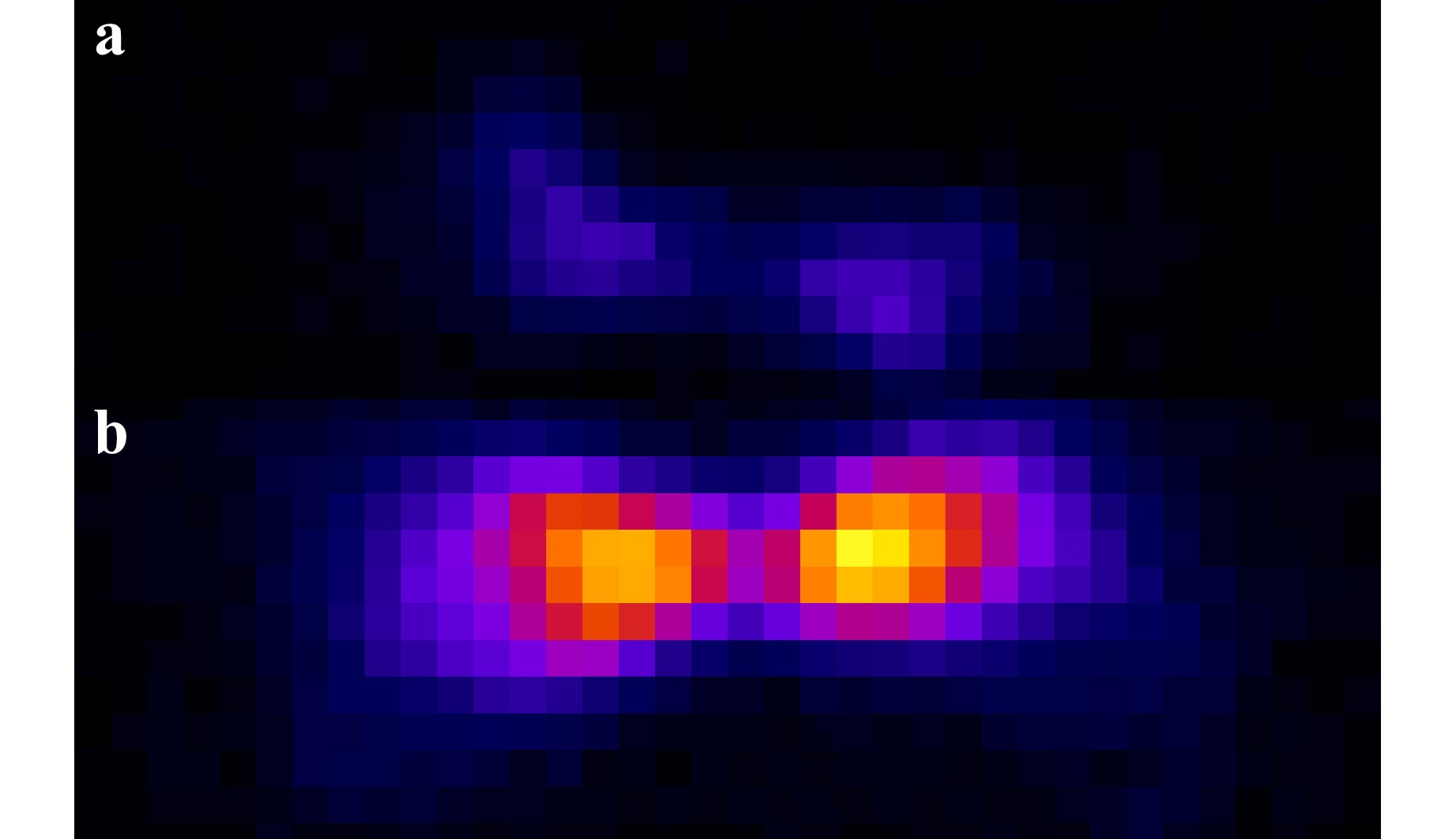
Fig. 4  Images of the same particle with a LCoS SLM a and the manufactured phase mask b for nearly identical experimental conditions. Both images are the mean of 250 frames to eliminate random noise. The peak brightness value is slightly more than 5 times higher with the manufactured phase mask.

from³⁵, where $ \Delta l $ is usually 2 for obtaining a point spread function with two maximums. Accordingly, the right side of this equation can be influenced with the parameters $ N $, $ R $ and $ f_1 $. $ N $ is the number of radial zones of the spiral phase mask, $ R $ is the radius of the phase mask and $ f_1 $ is the effective focal length of the optical setup between the measurement volume and the phase mask¹⁶.

The spatial phase-modulation of the light in the pupil plane can be achieved with a multitude of techniques. Often, Liquid crystal on silicon (LCoS) SLMs are employed for this^16,32,36 because they offer a convenient way to change the phase-modulation mask quickly and therefore offer a high flexibility for experiments. However, for fluorescence microscopy LCoS SLMs often decrease the light throughput substantially. The main reasons for this are firstly the restriction to one linear polarisation direction (50% loss for unpolarised fluorescent light) as well as the regular pixel grid, which results in diffraction of the light into several diffraction orders (40% loss for Holoeye Pluto 1 according to specification). An additional disadvantage of LCoS SLMs is that most of them are reflective elements and therefore require beam folding and a more precise alignment.

To circumvent these drawbacks, a transmissive custom phase mask was designed that was manufactured with Laser Direct Writing³⁷. Its properties are given in Table 1. The structured photoresist was directly utilized without further replication because at low quantities this would increase the costs without significant additional benefits. Fig. 4 and Table 2 show the comparison of light throughput and measurement uncertainty at nearly identical operating conditions with an inverse fluorescence microscope. It can be seen that the light efficiency is increased by a factor of slightly more than 5 whereas the axial random uncertainty is reduced by about 68%. Furthermore, the lateral uncertainty is reduced slightly by about 7%. Because the approximately linear relationship between the axial coordinate $ z $ and the orientation angle $ \psi $ is unambiguous for $ -90^\circ < \psi \leq +90^\circ $, the resulting relative uncertainty is about $ 0.13^\circ/180^\circ = 0.072{\text{%}} $. The prevalent reason for the significantly reduced axial uncertainty is probably the increased light efficiency. However, one reason for better performance might also be temporal noise that is introduced by the pulse-width modulation of the liquid-crystal cells³⁸.

In order to characterise the random uncertainty of the presented setup in Fig. 3 experimentally, the axial position of immobile fluorescent particles was measured for 250 subsequent frames. Accordingly, the random axial uncertainty was determined to be 27.5 µm for a measurement range of about 4000 µm (Fig. 5) at a frame rate of 800 Hz.

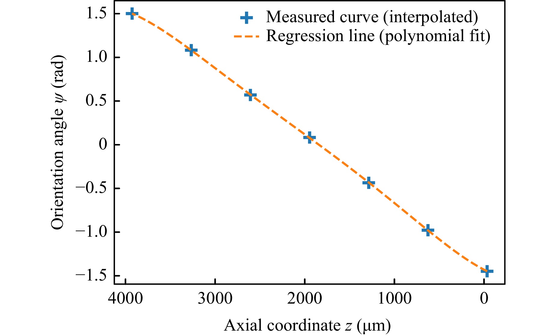
Fig. 5  Measured relationship between DH-PSF orientation angle $ \psi $ and axial coordinate $ z $. This calibration curve was similarly obtained as described in¹⁶.

A mathematical model of the adaptive optics system was developed for gaining a deeper understanding of it as well as optimisation and simulation. In the following, approximate equations are derived which describe the relationship between phase boundary shape, deformable mirror and wavefront measurement for the static case.

Fig. 6 shows a simplified optical illustration of the adaptive optics system. The goal of using the adaptive optics system is to correct wavefront disturbances that are introduced by refraction at the fluctuating phase boundary. This wave-optical approach can be translated to geometrical optics because the wave vector points locally in the propagation direction of equivalent light rays. Therefore, the model is derived using paraxial optics.

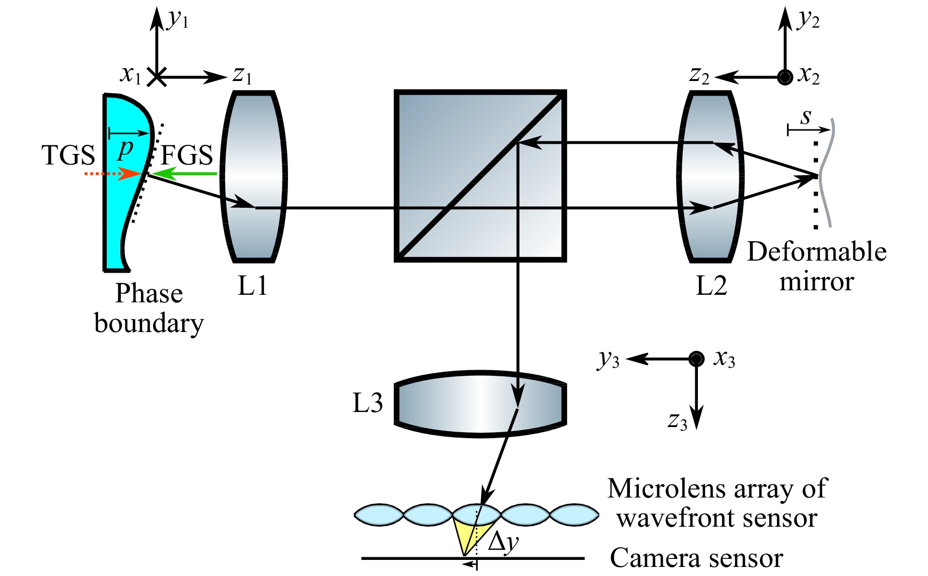
Fig. 6  Simplified optical setup for visualisation of relationship between phase boundary, deformable mirror and wavefront sensor output. The incident rays of the FGS are illustrated as green arrow. The reflected rays are imaged to the deformable mirror and then to the wavefront sensor. The resulting focal point displacement $ \Delta y $ on the camera sensor is directly related to the shape of the phase boundary and the deformable mirror. TGS: Refracted Light Beam, FGS: Reflected Light Beam

For a ray at the phase boundary position $ (x_{1,0}, y_{1,0}, z_{1,0} \approx 0) $ with the angles $ (\alpha_{x,1}, \alpha_{y,1}) $ (Fig. 7) the resulting ray at the wavefront sensor has the position $ (x_3', y_3') $ and the angles $ (\alpha_{x,3}', \alpha_{y,3}') $ (Fig. 8) given by equations 4 and 5.

Fig. 7  Sketch for visualisation of angle $ \alpha_{y,1} $ and position $ (x_{1,0}, y_{1,0}, z_{1,0}) $ of ray that starts at the phase boundary. The angle $ \alpha_{x,1} $ has an equivalent orientation to the coordinate system as $ \alpha_{y,1} $.

Fig. 8  Sketch for visualisation of angle $ \alpha_{y,3}' $ and position $ (x_{3,0}', y_{3,0}', z_{3,0}') $ of ray that arrives at the wavefront sensor. The angle $ \alpha_{x,3}' $ has an equivalent orientation to the coordinate system as $ \alpha_{y,3}' $. For explanation of $ \Delta y $, see Fig. 6.

$\, \beta_1 = - f_2/f_1 $ and $\, \beta_2 = - f_3/f_2 $ are the magnifications from the phase boundary to the deformable mirror (L1 and L2) and from there to the wavefront sensor (L2 and L3), respectively. $ \varphi_x $ and $ \varphi_y $ are the local tilt angles of the deformable mirror at the intersection point with the corresponding ray. It holds

where $ s(x_2, y_2) $ is the height of the deformable mirror at the position $ (x_2, y_2) $ (Fig. 6).

$ (\alpha_{x,1}, \alpha_{y,1}) $ depend differently on the local phase boundary tilt angle for refracted and reflected rays. For reflected rays it holds $ \alpha_{x/y,1,r} = -2 \theta_{x/y} $ for normal incidence, whereas for refracted rays $ \alpha_{x/y,1,t} = \arcsin((n_F/n_A) \cdot \sin(\theta_{x/y})) - \theta_{x/y} $ is found. A linear approximation gives

In the next considerations, $ \theta_{x/y,0} = 0 $ is assumed, which gives $ \alpha_{x/y,1,t} = + (n_F/n_A - 1) \cdot \theta_{x/y} $. $ n_F $ and $ n_A $ are the refractive indices of the fluid (in most cases water and air). $ \theta_x $ and $ \theta_y $ are defined as

where $ p(x_1, y_1) $ is the height of the phase boundary at the position $ (x_1, y_1) $ (Fig. 7).

With this model the correcting shape of the deformable mirror for a given phase boundary can be identified as

for small angles. The different sign for $ x_1 $ and $ y_1 $ is due to the different direction of the $ x_1 $ and $ x_2 $ axis. It can be seen that the correcting shape for refracted light is basically the phase boundary shape, but

1. laterally scaled by $ \,\beta_1 $, usually $\, \beta_1 < 0 $, and

2. axially scaled by $ - (\dfrac{n_F}{n_A} - 1)/ 2 $.

For $ |\,\beta_1| > 1 $ the slope of $ s_c(x_2, y_2) $ is smaller than that of $ p(x_1, y_1) $, meaning that the magnification $\, \beta_1 $ can be used to adjust the maximum mirror stroke to the maximum height of the phase boundary surface.

Furthermore, the relationship between the wavefront of a refracted light beam and a reflected light beam can be identified. In our previous publications^14,16 this relationship was found using an experimental parameter identification. The model makes it possible to find the system parameters that influence this relationship as well as their quantitative contribution. Accordingly, the relationship between the angles $ (\alpha_{x,3,r}',\alpha_{y,3,r}') $ of a reflected light beam and the angles $ (\alpha_{x,3,t}', \alpha_{y,3,t}') $ of a refracted light beam are related by

with $ k_t = (n_F/n_A - 1) $. Thus, it can be seen that only the parameters $ \,\beta_2, n_F $ and $ n_A $ influence this relationship. Furthermore, it becomes clear that $ (\varphi_x, \varphi_y) $ must be known for estimating $ (\alpha_{x,3,t}', \alpha_{y,3,t}') $ from $ (\alpha_{x,3,r}', \alpha_{y,3,r}') $. As a verification, $ k_t/2 $ was determined experimentally for a flat water surface. The measured value $ k_t/2 = 0.1755 \pm 5{{\% }}$ agrees well to the theoretical value $ 0.165 $.

If the phase boundary is statically curved, the assumption $ \theta_{x/y,0} = 0 $ is not valid. In this case, the linearisation in equation 8 results in a different slope $ k_t $ than $ n_F/n_A - 1 $. However, the dependence of $ k_t $ on $ \theta_{x/y,0} $ is quite small. Only for an angle of $ \theta_{x/y,0} > 17^\circ $ the error is larger than 5% if $ \theta_{x/y,0} = 0 $ is assumed. Therefore, the relationship between the refracted probe beam (TGS) and the reflected probe team (FGS) does not depend strongly on the static curvature of the phase boundary. Estimating the wavefront of the TGS with equation 12 and $ k_t = (n_F/n_A - 1) $ works sufficiently well even for statically curved boundaries.

To summarize, the derived model makes two things possible. Firstly, it describes the basic functionality of the adaptive optics system such as how to find the correcting mirror shape from the wavefront measurement of a light beam that was reflected at the liquid-gas interface. Secondly, it gives quantitative information about the influence of system parameters such as focal lengths.

In order to achieve a good correction quality, the instantaneous mirror shape must converge quickly and accurately to the desired correcting surface (Eq. 11), which is only possible if a sufficiently large number $ N_z $ of Zernike polynomials are controlled. However, the effort for technical realization increases with $ N_z $. Furthermore, it is unclear to which extent high order phase boundary oscillation modes need to be corrected, because usually the low-order modes have larger amplitudes³⁹. Therefore, it is helpful to analyse which Zernike polynomials are most important for the correction.

In order to identify the most prevalent contributions, the wavefront measurements of a fluctuating phase boundary were decomposed into Zernike polynomials for firstly an extended water surface, which is flat for no incident air flow, and secondly for a droplet. For that purpose, the movement of $ N_B $ focal points was recorded and stored in a $ N_t \times 2 N_B $ matrix $ U $, where $ N_t $ is the total number of time steps. The experimental parameters for the oscillating droplet are shown in Table 3 (see section 5), the experiment with the statically flat water surface was similar. Fig. 9 shows the relative signal energy contribution of the first 5 Zernike polynomials for the two different cases.

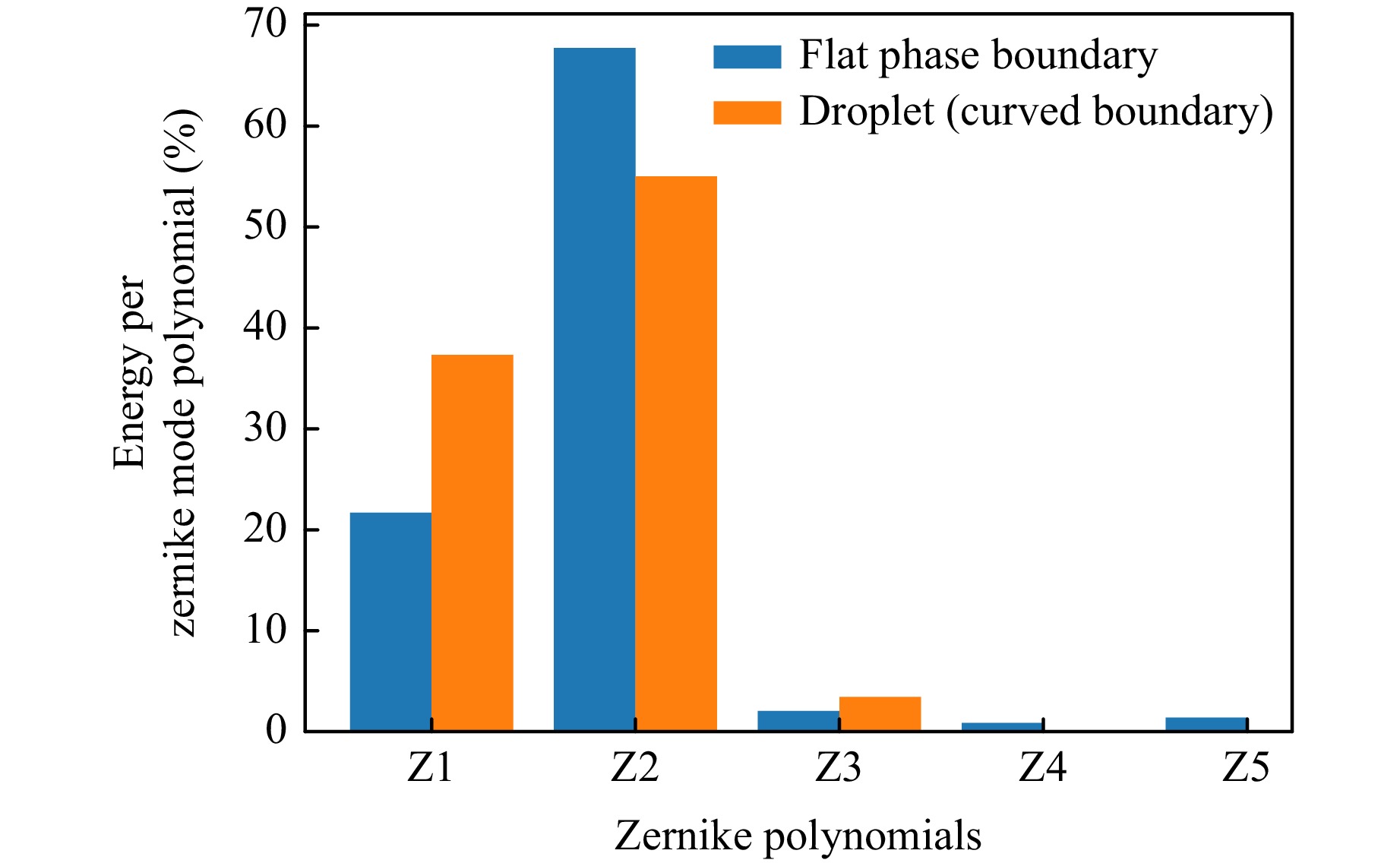
Fig. 9  Relative contribution of signal energy of the first five Zernike polynomials. Z1: tip, Z2: tilt, Z3: defocus, Z4/Z5: oblique and vertical astigmatism. The modes were obtained numerically from the measured wavefront sensor signal of an oscillating flat water surface as well as of a droplet.

In the case of an extended water surface $ N_B = 31 $ focal points were tracked on the Hartmann-Shack sensor. Despite theoretically $ 2 N_B = 62 $ degrees of freedom, it can be seen in Fig. 9 that the first two Zernike polynomials constitute about 90% of the total signal energy. Therefore, it can be assumed that two degrees of freedom are sufficient to describe the wavefront sensor output in this experiment reasonably well.

For a 50-µl droplet, the wavefront measurement with the Hartmann-Shack sensor is impeded by the strong static curvature (Fig. 10). $ N_B = 4 $ focal points are available at the droplet center because at this position the local tangent plane of the phase boundary is approximately horizontal. Outside the center of the droplet, the reflected light rays of the FGS exhibit a large angle towards the optical axis and are therefore no longer captured by the optical system due to the limited numerical aperture, so that as a result the corresponding subapertures are dark. Therefore, the coefficients of higher Zernike polynomials than Z3 are not available in this case.

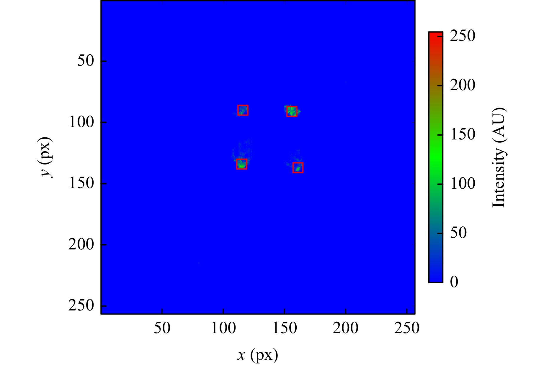
Fig. 10  Hartmannogram of a 50-µl droplet. The static curvature of the phase boundary reduces the Hartmann-Shack image to 4 spots, which corresponds to a field of view of about 500µm × 500µm at the droplet surface for the adaptive optics system. The red rectangles around the focal spots denote the successful tracking.

The reason for this is the finite Helmholtz-Lagrange invariant of the optical system which constitutes a trade-off between the size of the FOV and the maximum light ray angle that is still captured by the system (numerical aperture). Because the reflected rays have an angle of $ \alpha_{x/y,1,r} = -2 \theta_{x/y} $ (see section 3), the system is quite sensitive to static curvatures $ \theta_{x/y,\text{stat}} $ of the liquid-gas interface. However, because tip and tilt contain also in this case about 90% of signal energy (Fig. 9), it can be assumed that this limitation does still allow us to correct the most prevalent oscillation modes. In future work, it is planned to optimise the wavefront sensor by increasing the Helmholtz-Lagrange invariant, so that a large FOV can be achieved in presence of a significant surface curvature.

The reason for the prevalence of tip and tilt is presumably that the field of view of the wavefront sensor is small compared to the characteristic length of the oscillation modes, which is the wavelength of the capillary-gravity waves. It can be assumed that this is the case for many measurement scenarios in microfluidics. However, there may be cases where more Zernike polynomials are needed, for example because the oscillation modes are different or because the FOV of the adaptive optics system is larger.

In order to characterise the correction performance of the adaptive optics setup, the virtual movement of immobile particles caused by the refraction at the oscillating phase boundary was analyzed with and without correction (Fig. 11). Immobile particles were fixed to the gas diffusion layer and used as a reference for a quantitative measurement of the uncertainty due to dynamic aberrations. The particles were fixed by applying distilled water with particles to the GDL. After evaporation, the particles still adhere to the GDL even if the droplet for the experiment is applied with a micropipettor. During the experiment, a grazing air flow induced an oscillation of the droplet with a characteristic rocking motion, that is governed by the first and second eigenfrequency of the droplet. The parameters of the experiment are shown in Table 3. In respect to the results of section 4, the first two Zernike polynomials tip and tilt were corrected. The evaporation of the droplet was found to be negligible compared to the measurement time because at maximum laser power it took 40min until about 85% of the droplet was evaporated.

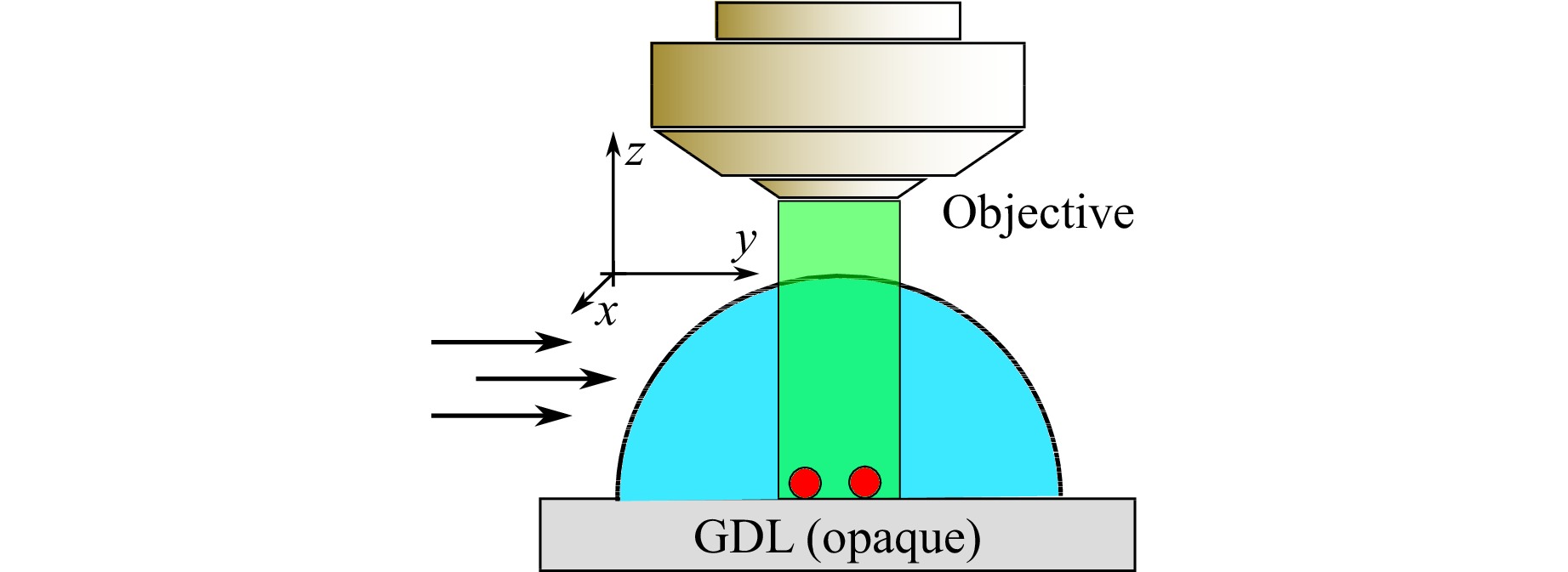
Fig. 11  Sketch of experimental setup for characterising the correction performance of adaptive optics. An airflow from a nozzle induces a slight oscillation of the droplet. The orientation of the air flow arrows and the coordinate system is not for scale.

Fig. 12 shows an example power density spectrum (PDS) of the measured particle positions. The distinct eigenfrequencies of the droplet - which are given by the semi-empirical law 13 from⁴⁰ - are well visible in the spectrum.

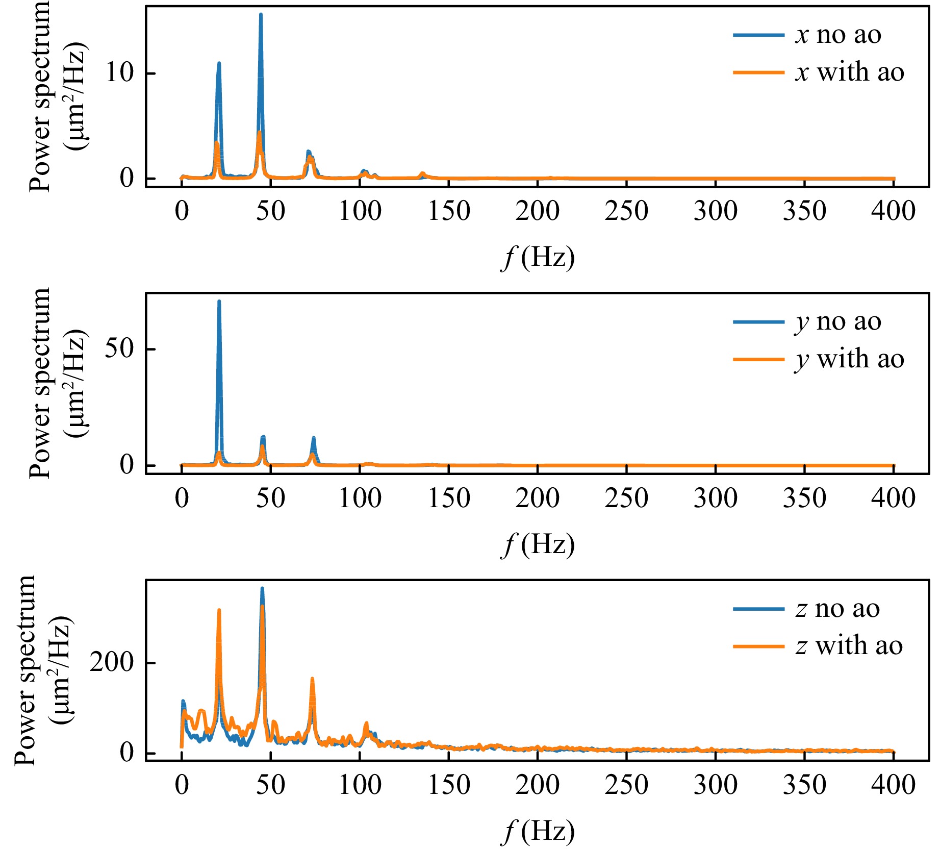
Fig. 12  Example PDS of immobile particle positions with and without adaptive optics. It can clearly be seen that the correction reduces the disturbance.

where $ \gamma = 71.69\;{\rm mN/m} $ is the surface tension, $ \theta = 94^\circ $ is the contact angle and $ m = 50\;{\rm mg} $ is the droplet mass. Furthermore, it can clearly be seen that the total power of the disturbance is reduced if the correction is applied, especially for the first eigenfrequency at circa 21 Hz.

Fig. 13 and 14 show the random position uncertainty averaged over 5 experiments. Although the lateral uncertainty is corrected by 58.5% for the first eigenfrequency, this is not the case for the axial position uncertainty. It can be assumed that the reason for this are oscillation modes of the water-air boundary which are not measured by the wavefront sensor, otherwise these modes would be clearly detectable in the sensor signal and tip/tilt would not account for 92% of signal energy. Although theoretically the reason for this could be quite complicated wave shapes, it is more likely that an (in combination with tip and tilt occuring) axial displacement of the water-air boundary is the reason for this (Fig. 15). Because the Hartmann-Shack wavefront sensor can only measure the derivative of the phase boundary, this axial displacement can not be detected. The observed position $ z_o $ is according to Fig. 15

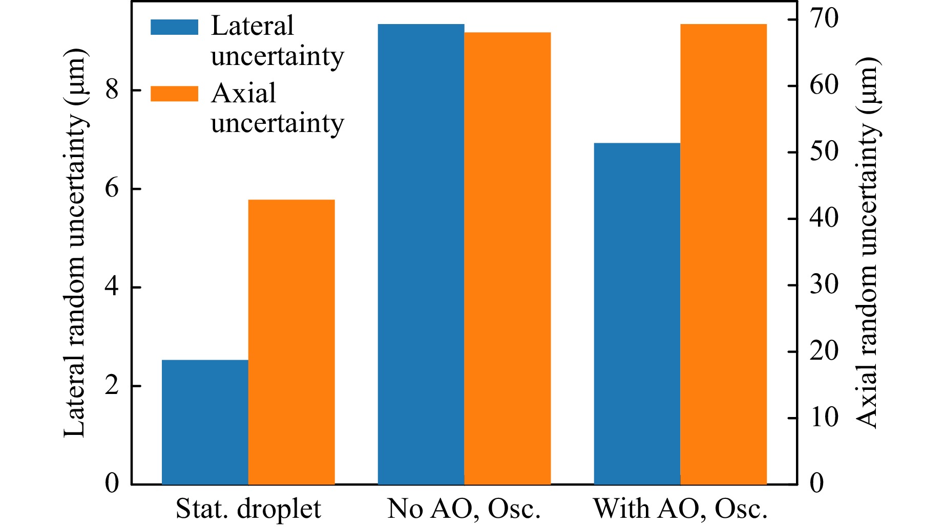
Fig. 13  Mean random uncertainty of 5 experiments. The uncertainty corresponding caused by the fluctuating interface is reduced by 28.3%.

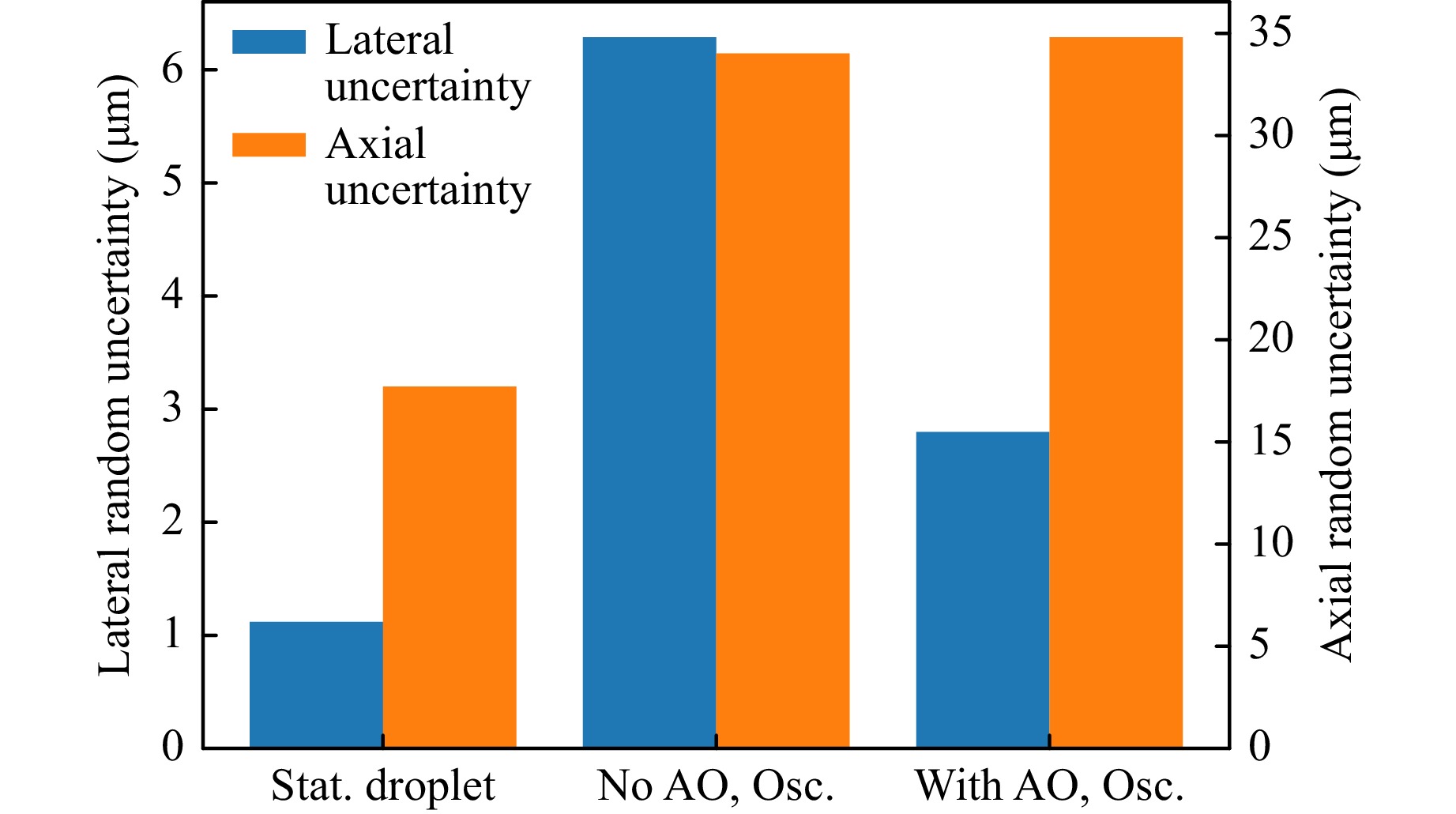
Fig. 14  Mean random uncertainty of 5 experiments for frequencies below 31Hz (only first eigenfrequency). The uncertainty corresponding caused by the fluctuating interface is reduced by 58.5%.

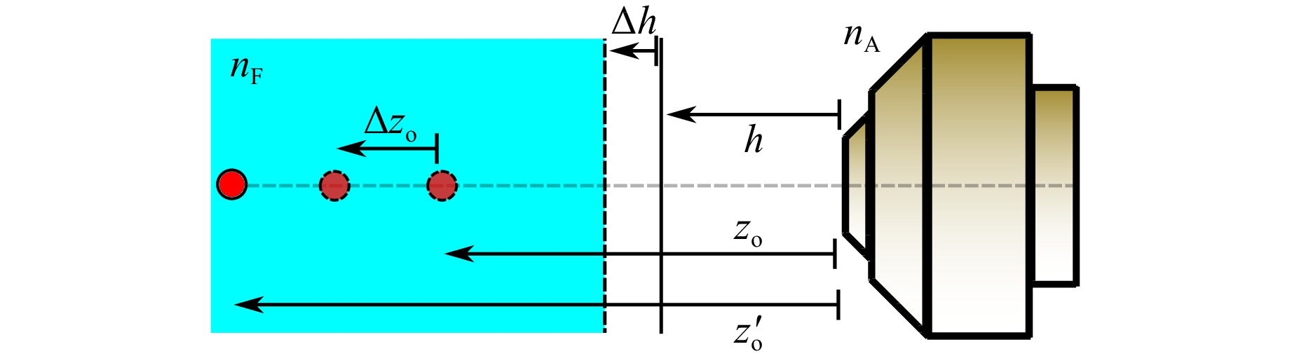
Fig. 15  Sketch for illustrating the influence of an axial displacement (along the z-axis) of the phase boundary on the particle localisation. $ h $ is the distance between objective and phase boundary in the static case. The particle has the real position $ z_o' $, but due to refraction at the phase boundary it seems as if the particle is located at $ z_o $. A change of $ \Delta h $ causes the observed position to change by $ \Delta z_o $.

where $ z_o' $ is the real position of the particle and $ h $ the water height. If the water level does not change ($ h $ is constant), the real position $ z_0' $ can be found - except for a constant offset - by multiplying $ z_0 $ by $ n_F/n_A $. However, if the phase boundary is axially displaced by $ \Delta h $, the measured change $ \Delta z_{o,\text{measured}}' $ of the observed position is accordingly

where $ \Delta h $ is the displacement of the water surface relative to the static position. According to equation 15 the increase in measurement uncertaninty by 25.2 µm (Fig. 13) corresponds to an oscillating axial displacement of $ \sigma_h = n_A/(n_F - n_A) \cdot \sqrt{(68\;{\text{µm}})^2 - (42.3\;{\text {µm}})^2} \approx 160\;{\text {µm}} $, which is plausible. In future work it is planned to modify the wavefront sensor so that this axial displacement can be measured.

In order to investigate the influence of aberrations on the flow measurement, the virtual motion of immobile and mobile particles near the GDL was compared with and without adaptive optics. The basic idea is that if the height difference between the mobile and immobile particles is sufficiently small, both particles will experience a similar virtual displacement due to the dynamical aberrations. In this special case, the virtual particle motion can be measured with the immobile particles. Afterwards, the measured motion of the mobile particles can be decomposed into motion due to the fluctuating water interface and motion due to the flow itself, because the former is known. In principle this experiment is similar to the experiment outlined in section 5, however, mobile particles that follow the flow were added to the droplet. The experiment parameters can be found in Table 4. The sketch can be seen in Fig. 16.

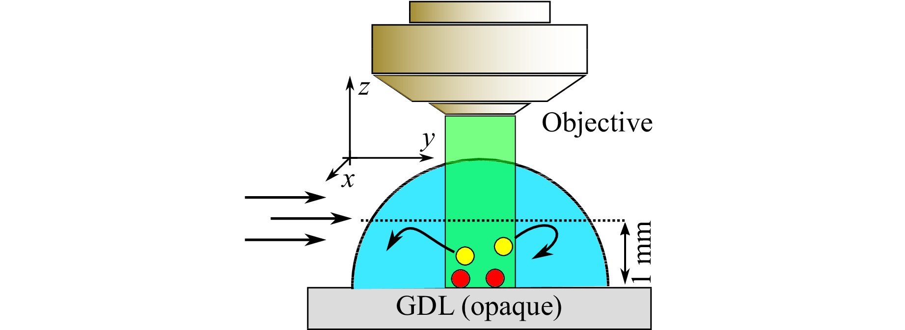
Fig. 16  Sketch of experimental setup for characterising the influence of the dynamic aberrations on the measured trajectories of the mobile trajectories. Red Points: Immobile Particles, Yellow Points: Mobile particles. The orientation of the air flow arrows and the coordinate system is not for scale.

For the evaluation, only trajectories with a maximum distance of ca. 1 mm to the GDL were selected. These trajectories were classified as immobile and mobile trajectories by comprising maximum covered distance as well as the manually given positions of immobile particles on the ground. The mean trajectory of the immobile particles was compared with the mean mobile particle trajectories. For isolating the first eigenfrequency, both signals were filtered using a low-pass FIR filter (Kaiser window) with a cut-off frequency of 35 Hz. Because this filter type has a linear-phase response, the fundamental signal form is not changed. As can be seen in Fig. 17, mobile and immobile particles seem to oscillate with a phase shift of about 180° if no correction is enabled. The mean Pearson correlation coefficients from all mobile trajectories with sufficient length of 6 different droplets are $ \bar{\rho}_x = -0.8621 $ (Standard deviation $ \sigma_{\rho} = 0.102 $) and $ \bar{\rho}_y = -0.7791 $ ($ \sigma_{\rho} = 0.1168 $) for the lateral dimensions. This confirms Fig. 17 quantitatively because a correlation coefficient of -1 indicates an inverse relationship.

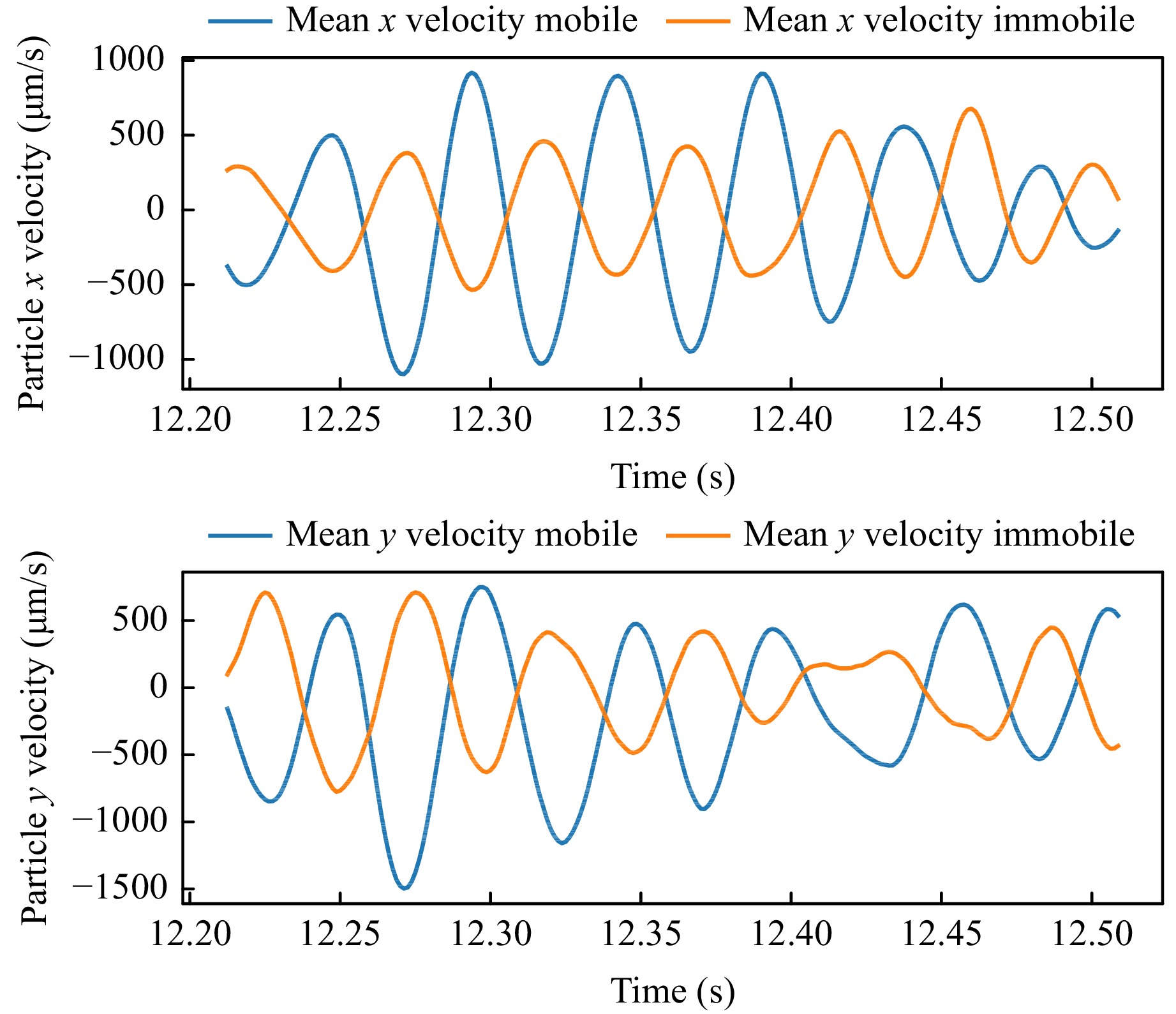
Fig. 17  Example plot for comparing the mean mobile trajectory (near the GDL) with the mean trajectory of the immobile particles. Both signals have been low-pass filtered to isolate the first eigenfrequency. The inverse relationship between both trajectories can easily be seen.

Fig. 18 suggests an explanation for this behaviour. From recent literature⁴¹ it is known that the first eigenmode corresponds to a fluid movement from lee- to luv-side and vice versa. We assume that this refraction of light at the changing slope of the surface causes a seemingly displacement of the immobile particles in the opposite direction of oscillation. Although the mobile particles also experience this virtual displacement, the displacement due to the flow (that corresponds to this first eigenmode) is larger. Therefore, mobile and immobile particles seem to oscillate inversely (Fig. 17).

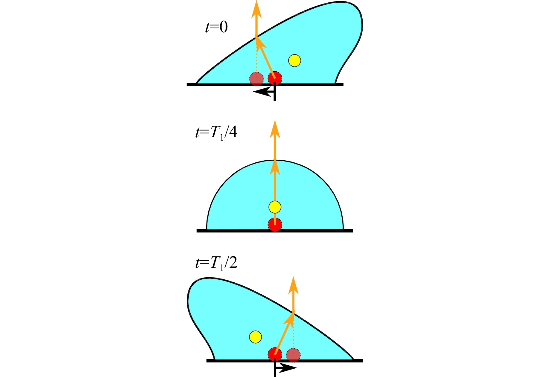
Fig. 18  Explanation for inverse relationship between measured immobile (red) and mobile (yellow) particle trajectories for the first eigenfrequency. The principal ray corresponding to the immobile particle is refracted at the phase boundary so that it seems as if this particle moves in opposite direction to the oscillation. Because almost all microscope objectives are objectside-telecentric^42,43, the prinicpal ray must be parallel to the optical axis outside the droplet. The light refraction of the mobile particle is not illustrated.

For flow measurements, only the movement of the mobile particles is relevant. In this case, the virtual displacement of the mobile particles due to the dynamical aberrations causes an underestimation of the oscillation magnitude of the first eigenmode. This can be easily recognized in Fig. 17, because for the mobile particle, the true motion (without dyn. aberrations) can be approximated by subtracting the immobile particle's trajectory. Accordingly, the flow measurement exhibits a systematic error without correction.

For verifying this hypothesis, the same evaluation was repeated for the measured trajectories with active correction. Fig. 19 shows the mean tracer particle velocity PDS without and with adaptive optics. This spectrum was obtained by firstly calculating the PDSs of the mean mobile particle velocity for every experiment, and secondly averaging the PDSs of 6 different experiments. As expected, the magnitude of the first eigenfrequency is significantly underestimated without adaptive optics correction.

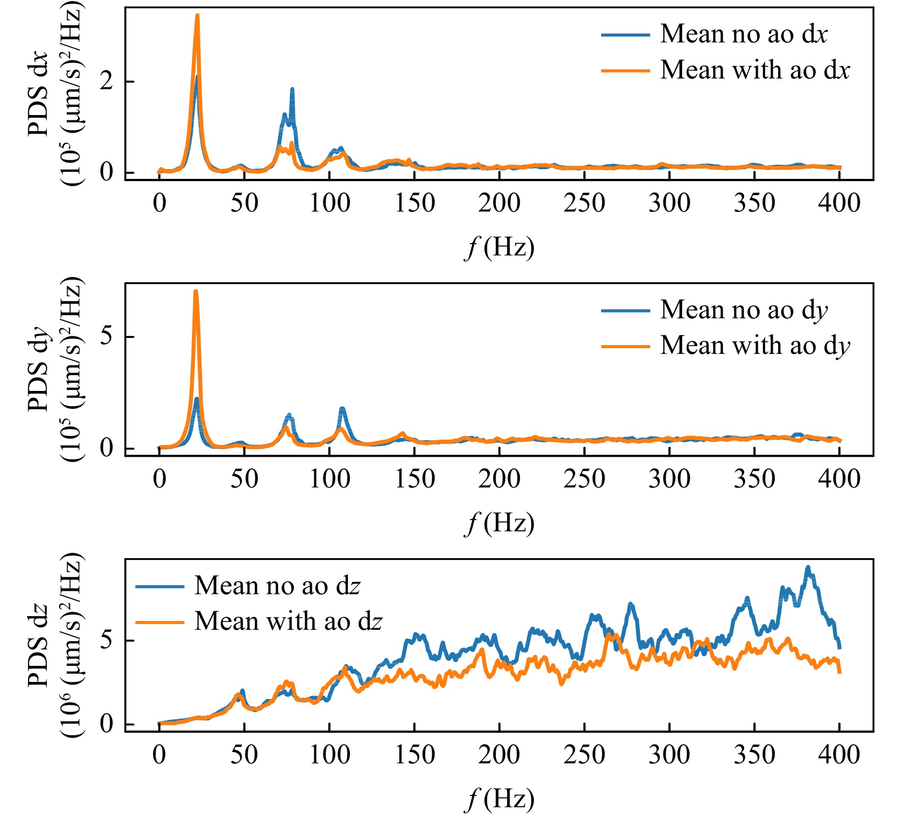
Fig. 19  Mean power density spectrum of mobile particle velocity averaged over 6 experiments. Only mobile particles with a maximum distance of about ca. 1mm to the GDL are included. It can be seen that the first eigenfrequency is significantly more pronounced with adaptive optics.

This mean spectrum offers a good qualitative comparison, but for quantitative analysis the results from single experiments are better suited because the eigenfrequencies and their magnitudes vary slightly between different experiments. Accordingly, the signal power was calculated by integrating the area of the first eigenfrequency peak in the power density spectrum individually for every experiment. Fig. 20 illustrates the relative power change with and without correction. It can be seen that the measured signal power of the first eigenfrequency is increased by about 70% if adaptive optics is active.

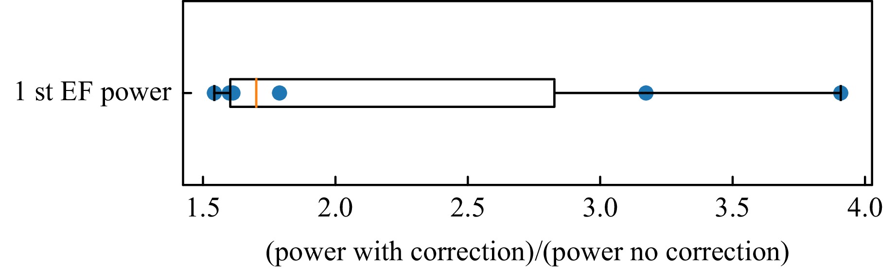
Fig. 20  Relative change of measured power of first eigenfrequency with and without adaptive optics. It can be seen that with adaptive optics the first eigenfrequency is more pronounced. Hence, the systematic error due to dynamic aberrations is reduced.

For higher eigenfrequencies, quantitative analysis is more difficult because their lower relative power makes their detection more difficult. However, for the 4th eigenfrequency ($ f_5 \approx 76\;{\rm Hz} $) the adaptive optics correction lowers the power contribution to the measured mobile trajectory in average by 50% to 60%.

The axial $ z $-component of the mobile particles reveals two distinct eigenfrequencies as well: $ f \approx 49\;{\rm Hz} $ and $ f_5 \approx 76\;{\rm Hz} $. However, similar to the results in section 5, the adaptive optics correction does not have much influence. Because the random measurement uncertainty for the axial position is higher than for the lateral dimensions, and because the numerical differentiation of the position signal acts as a high-pass filter, the z-spectrum exhibits a significantly higher noise level, especially for higher frequencies.

The underestimation of the first eigenfrequency magnitude and its correction with the adaptive optics system can not only be seen in the particle velocity spectrum (Fig. 19), but it is also possible to visualise this effect spatially resolved. Fig. 21 shows the measured periodic flow field corresponding to the first eigenfrequency with and without adaptive optics. The experimental conditions are identical to those presented in Table 4. It can be seen that the flow field changes periodically between flow to the bottom left and bottom right. Furthermore, the flow field comparison shows that the flow magnitude is significantly larger with active correction due to reasons previously discussed.

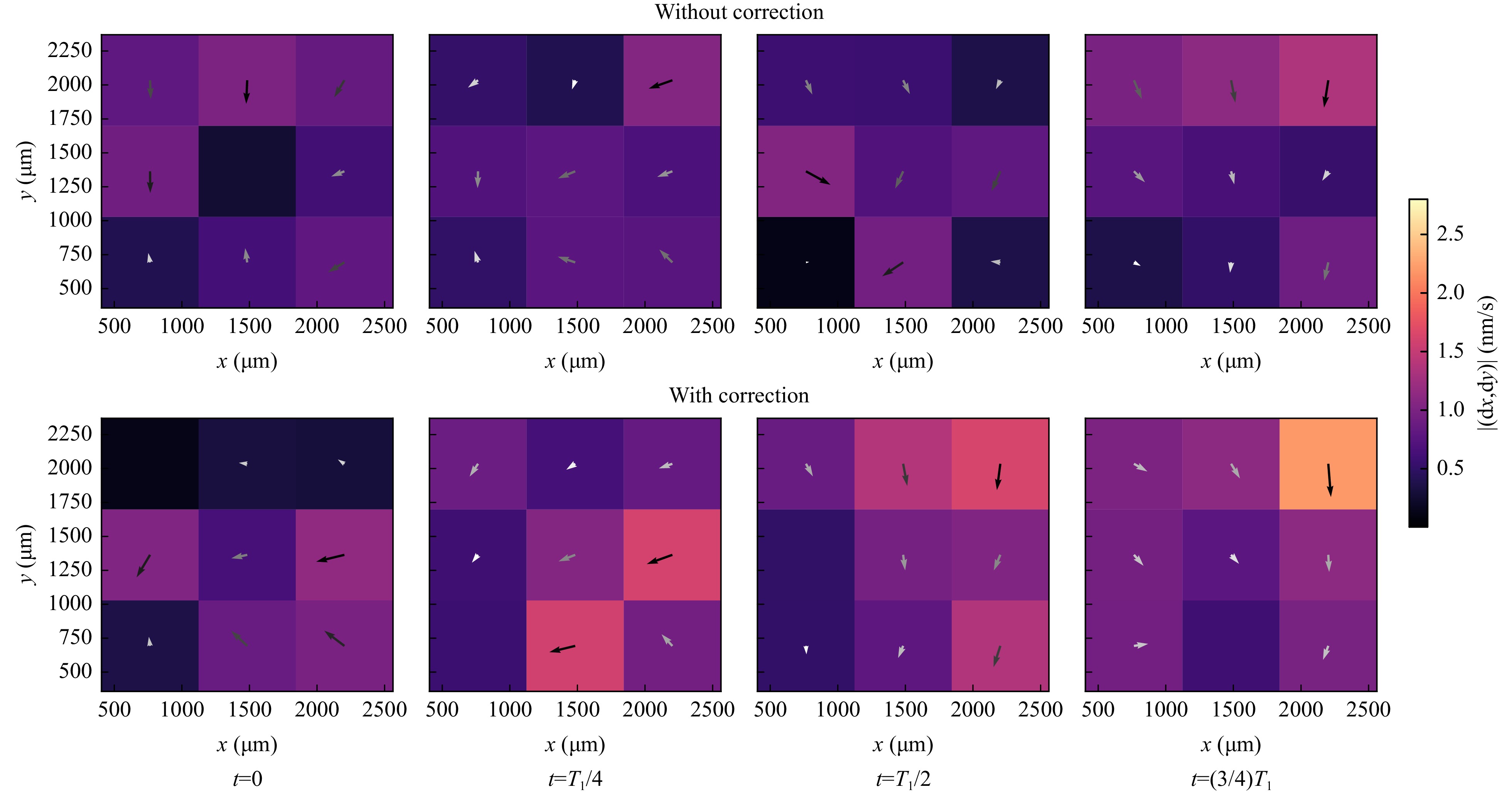
Fig. 21  Phase-averaged measurement of flow field between GDL and up to ca. 1mm above it for the first eigenfrequency. The flow field was measured in the center of the droplet. Top row: No adaptive optics, Bottom row: With adaptive optics. It can be seen that the flow velocity of this oscillation is significantly underestimated if no adaptive optics is used.

The phase-averaged flow field was obtained by applying a lowpass filter ($ f_{\text{cut}} = 30\;{\rm Hz} $) to the individual mobile particle trajectories where the filtering was achieved by applying a Chebyshev type I filter (Order = 6) forwards and backwards, respectively. This approach yields a zero phase filter so that the original signal form is not changed. After that, the individual vectors (which form the trajectories) were subsequently binned and averaged for every interrogation window.

Multiphase flows occur in many manufacturing applications, however there is still a lack of sufficiently good models and experimental data for predicting their behaviour. One of the main reason for this is that optical flow measurements are significantly impaired if the only optical access is a fluctuating liquid-gas interface. The temporally-varying refraction of light introduces dynamical aberrations which result in a larger measurement uncertainty (which includes random as well as systematic errors).

In this manuscript, a solution based on adaptive optics for reducing this uncertainty was presented. Firstly, the optical setup and the closed-loop control concept were introduced. A custom manufactured phase mask increased the light efficiency by a factor of 2.5 compared to a LCoS SLM (for one polarisation direction) and thus enabled the measurement at sufficiently high frame rates (800Hz). In the following, a mathematical model was derived that describes the Hartmann-Shack sensor measurement as a function of phase boundary and mirror shape. This model indicates that for estimating the phase boundary slope from the Hartmann-Shack sensor measurement approximately only the optical magnification as well as the refractive indices of the gaseous and the liquid medium are necessary. Afterwards, a time series of wavefront sensor measurements was decomposed into orthogonal Zernike polynomials for a fluctuating (mostly) flat water-air surface and for a droplet which revealed that a tip and tilt motion of the phase boundary accounts for most of the dynamical aberrations. The reason for this is presumably that the characteristic length of the water waves is relatively large compared to the field of view of the wavefront sensor for the investigated experimental conditions. In future, this finding can be used to simplify the setup by substituting the deformable mirror for a fast-steering mirror, so that costs and complexity can be reduced. Subsequently, the correction performance of the adaptive optics setup was characterised for 50-µl droplets on a GDL substrate utilizing fixed, immobile fluorescent particles. It was shown that the uncertainty caused by the fluctuating interface is reduced by 58.5% for the first eigenfrequency. In the following, the influence of the dynamic aberrations on flow measurements was characterised. We found that the temporally varying refraction at the water-air interface introduces a systematic underestimation of the flow oscillation amplitude (of the first eigenmode). Eventually, it was demonstrated that the adaptive optics setup reduces this underestimation so that the phase-averaged flow of the first eigenmode can be measured accurately. Because the first eigenfrequency is particularly important for the detachment of sessile droplets, the ability to measure it precisely is the key to more accurate droplet motion models. Such models can then be used for optimising technical systems, for instance for improving the droplet removal in fuel cells. The ability to investigate the flow even in droplets on opaque surfaces is particularly important as most surfaces in technical applications are opaque (e. g. GDL, structured steel, etc.).

In future work, it is planned to apply the adaptive optics correction to other measurement objects like bubbles or film flows. Furthermore, the correction will be extended so that axial displacements of the phase boundary can be measured. We assume that the presented technique has a high potential for finding new fluid mechanical insights, especially because to our knowledge no other correction technique for flow measurements through fluctuating interfaces exists.

The authors would like to sincerely thank Christof Pruß (ITO Stuttgart) for manufacturing the phase mask (section 2). Furthermore, we wish to express our gratitude to Dr. Felix Schmieder for his expertise and advice. Additionally, we thank Dr. Johannes Gürtler for providing us the Phantom high-speed camera, although it is a crucial component for his research. The research project IGF-Nr. 21190 BG/2 from the research association DECHEMA e. V. is supported by the Federal Ministry of Economic Affairs and Energy through the German Federation of Industrial Research Associations (AiF) as part of the programme for promoting industrial cooperative research (IGF) on the basis of a decision by the German Bundestag. Furthermore, this work is partially supported by the Deutsche Forschungsgemeinschaft (DFG, German Research Foundation) - BU 2241/6-1.