A comprehensive review of dwell time optimization methods in computer-controlled optical surfacing

Over the past decade, precision machining technologies have rapidly developed, resulting in the increased amount of high-end optics in various applications such as telescopes for space exploration^{1, 2}, extreme ultraviolet (EUV) lithography systems^{3, 4}, synchrotron radiation and free-electron laser beamlines^{5, 6}, and more. These optics require stringent specifications on surface precision and aspherical surface shapes to better compensate for aberrations⁶ and adapt to compact designs^{2, 7}, which has led to the invalidation of conventional mechanical polishing methods and the emergence of computer-controlled optical surfacing (CCOS) technologies^{8, 9}. Nowadays, most precision optical surfaces are manufactured using CCOS processes, which rely on computer control of machine tools to correct errors on an optical surface in a deterministic manner. The machine tool used in CCOS systems is much smaller than the clear aperture (CA), or effective area, within an optical surface, effectively reducing any local errors with feature sizes smaller than the machine tool stroke.

Since its inception by Jones in the 1970s¹⁰, numerous CCOS processes have been developed, including small-tool polishing^{11, 12}, bonnet polishing^13-15, magnetorheological finishing^16-18, ion beam figuring (IBF)^19-21, and fluid jet polishing (FJP)^22-24. The choice of CCOS processes largely depends on the precision and target shape of the optical surfaces.

A typical CCOS process comprises a metrology-and-fabrication loop, as illustrated in Fig. 1, where $ {\bf{x}}=(x,y) $ is the surface coordinates. During the metrology phase, the actual surface shape $ z_{a}\left({\bf{x}}\right) $ is measured. The current surface error $ z_{e}\left({\bf{x}}\right) $ is calculated as the difference between $ z_{a}\left({\bf{x}}\right) $ and the target surface shape $ z_{t}\left({\bf{x}}\right) $. Combined with the Tool Influence Function (TIF) $ r({\bf{x}}) $ extracted from the machine tool and the pre-defined tool path $ {\bf{u}}=\left(u,v\right) $, a dwell time distribution $ t\left({\bf{u}}\right) $ is calculated, which is then converted to and fed as velocities $ v\left({\bf{u}}\right) $ in a Computer-Aided Manufacturing (CAM) software. This velocity distribution is then utilized to estimate the residual error $ z_{r}^{est}\left({\bf{x}}\right) $ and guide the motion of the machine tool over the optical surface to remove material. After each machining cycle, a new $ z_{e}\left({\bf{x}}\right) $ is measured and compared to $ z_{r}^{est}\left({\bf{x}}\right) $ to confirm the convergence of the process and determine if the target residual error requirement is satisfied.

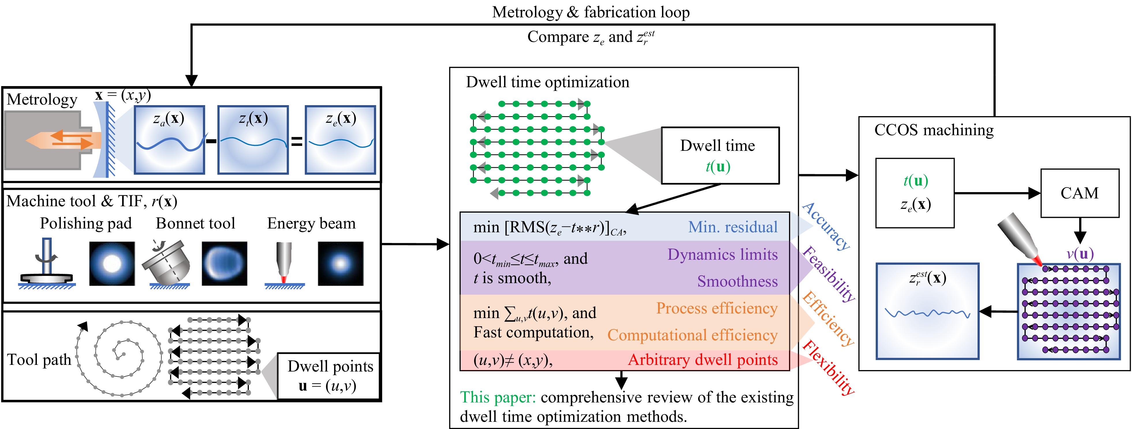
Fig. 1  An iterative CCOS process is composed of metrology, machine tool influence function extraction, tool path planning, dwell time optimization and CCOS machining.

As shown in Fig. 1, the dwell time quality directly impacts the accuracy and convergence of a CCOS process. The dwell time solution is derived from Preston’s equation²⁵, which models material removal per unit of time as

where $ {\dot z}\left({\bf{x}};t\right) $ is the partial derivative of $ z({\bf{x}};t) $ with respect to $ t $, $ \kappa $ is the Preston constant determined by the process parameters such as the material of the surface and abrasives, $ s\left({\bf{x}};t\right) $ and $ f\left({\bf{x}};t\right) $ are the pressure and relative velocity between the tool and the workpiece at the point $ {\bf{x}} $. By integrating Eq. 1 with respect to time and treating $ \kappa\cdot s\left({\bf{x}};t\right)\cdot f\left({\bf{x}};t\right) $ as a static TIF, in which $ t $ can be neglected, i.e. $ r\left({\bf{x}}\right)=\kappa\cdot s\left({\bf{x}}\right)\cdot f\left({\bf{x}}\right) $, a two-dimensional (2D) convolutional material removal model^{8, 10} is obtained, where the removed material $ z\left({\bf{x}}\right) $ is modeled as the convolution between the static TIF $ r\left({\bf{x}}\right) $ and the dwell time $ t\left({\bf{x}}\right) $, given by:

where “$ ** $” denotes the 2D convolution operation. Eq. 2 is also called a linear and shift-invariant system, where the TIF is assumed to be temporally and spatially stable, and the material removal is linear with respect to the dwell time. Replacing $ z\left({\bf{x}}\right) $ by $ z_{e}\left({\bf{x}}\right) $ in Eq. 2, $ t\left({\bf{x}}\right) $ can be estimated through deconvolution. However, since deconvolution is an ill-posed inverse problem without a unique solution, $ t\left({\bf{x}}\right) $ can only be obtained by optimization. The field of 2D deconvolution has been widely explored in image super-resolution²⁶ and restoration²⁷, and many of the practical concepts have been applied to dwell time optimization^{10, 20, 28}. Nonetheless, as highlighted in Fig. 1, dwell time optimization has specific objectives that differ from those of image restoration and super-resolution.

● Accuracy: Image restoration and dwell time optimization approaches aim to minimize the residual error between the actual signal and the deconvolved signal. However, dwell time optimization focuses on minimizing the residual error in the CA, $ [z_{e}\left({\bf{x}}\right)-r\left({\bf{x}}\right)** t\left({\bf{x}}\right)]_{CA} $, where $ [\cdot]_{CA} $ denotes an argument in the CA.

● Feasibility: Two aspects should be considered to make the optimization feasible for actual fabrication: 1) Positivity and dynamics limits considerations. It is important to note that the dwell time $ t\left({\bf{x}}\right) $ should always be positive and constrained by $ t_{min} $ and $ t_{max} $, where $ 0<t_{min}\leq t\left({\bf{x}}\right)\leq t_{max} $, since most CCOS processes are material removal processes. These constraints are unnecessary for general image deconvolution. Also, the lower and upper limits, $ t_{min} $ and $ t_{max} $, respectively, indicate that the optimization of dwell time must consider the constrains of machine dynamics, such as maximum speeds and accelerations^{29, 30}. 2) Smoothness. The restored image in image deconvolution contains more details (i.e., higher-frequency components) than the captured image. However, in the optimization of dwell time, $ t\left({\bf{x}}\right) $ must smoothly duplicate the shape of $ z_{e}\left({\bf{x}}\right) $³¹. Any higher-frequency components are not expected in a dwell time solution, as they may result in frequent accelerations and decelerations that could compromise the stability of the CCOS process³². These two aspects together define the feasibility of a dwell time solution.

● Efficiency: Efficiency is composed of process efficiency and computational efficiency. 1) Achieving the target residual error with the shortest possible total dwell time is crucial to ensure process efficiency, particularly in large optics fabrication, which can take months or years to complete². 2) the computational cost of obtaining a valid dwell time solution must also be reasonable.

● Flexibility: As shown in Fig. 1, the dwell points $ {\bf{u}} $ are expected to be freely distributed over the surface coordinates $ {\bf{x}} $. This is different from image deconvolution, where the coordinates of the actual image and the restored image overlap with each other. The flexibility of having arbitrary dwell points is essential, as it enables the usage of advanced tool paths^33-35 to reduce the generation of periodic, middle-frequency errors, which can be hard to remove³⁶.

In actual CCOS processes, achieving all these objectives simultaneously is challenging. The machine dynamics constraints, for instance, can affect the accuracy of the process since the planned dwell time may not be realizable by the machine. While it is possible to optimize the machining process for minimized middle-frequency errors and maximum efficiency by carefully selecting the dwell points, this may impact the overall accuracy and incur additional computation cost. Therefore, a balance must be struck among accuracy, feasibility, efficiency, and flexibility.

Researchers have proposed a range of dwell time optimization methods to address the challenge of achieving the various objectives in CCOS processes. We classify these methods into two categories, namely the function-form and matrix-form methods, as illustrated in Fig. 2. Each category addresses different scenarios and distributions of dwell points relative to the surface coordinate grid, x, defined by the optical surface. The function-form methods directly tackle the convolution function in Eq. 2 under the assumption that the dwell points are distributed on the same coordinate grid defined by the surface. The matrix-form methods handle the cases in which the dwell points are arbitrarily distributed by discretizing Eq. 2 as

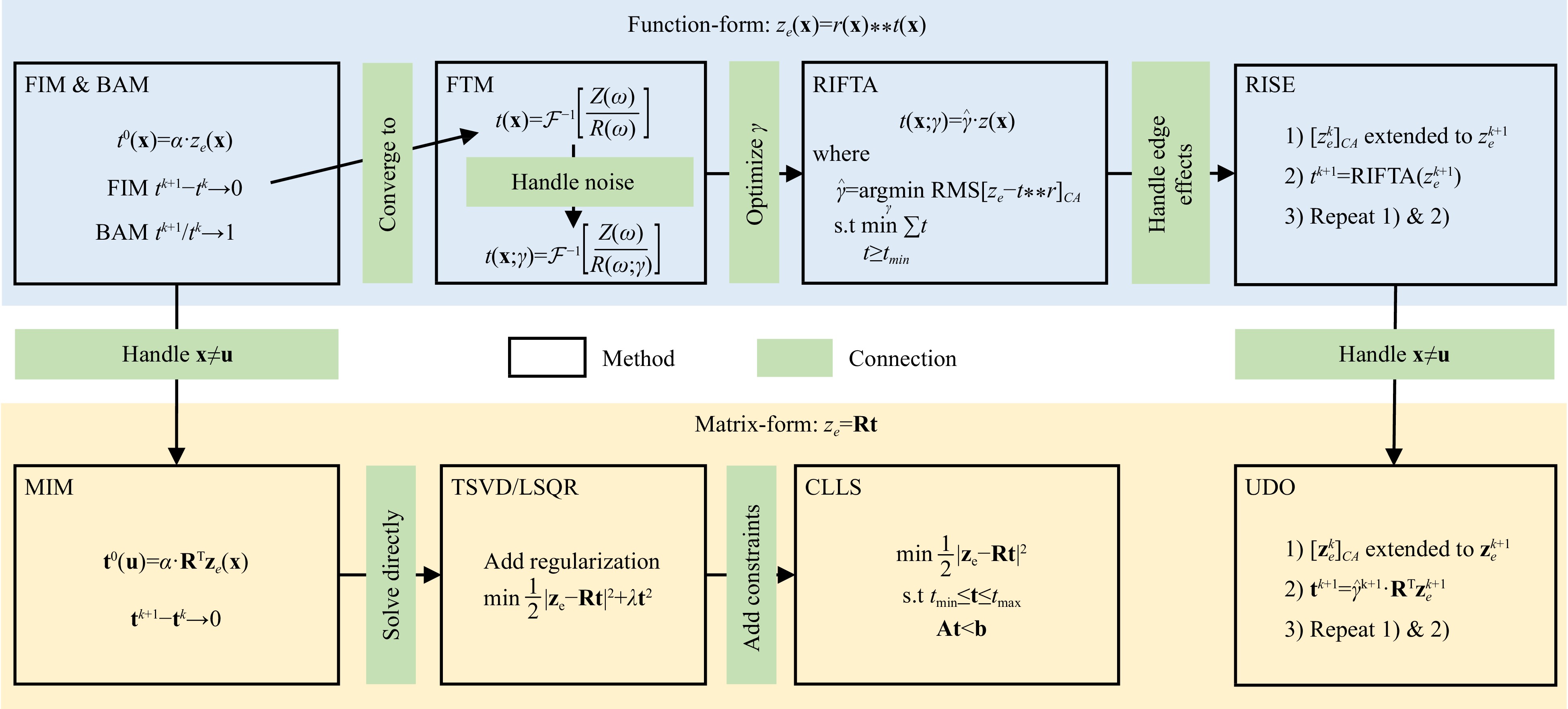
Fig. 2  Links among the existing dwell time optimization methods, where $ {\cal{F}}^{-1} $ denotes inverse Fourier transform, $ \alpha $ and $ \gamma $ are constant scalars, and $ {\boldsymbol{\omega}} $ denotes the frequency components.

for $ j=0,1,...,N_{z}-1 $, where $ N_{z} $ is the number of elements in $ z_{e}\left({\bf{x}}_{j}\right) $, $ N_{t} $ is the number of dwell points, $ {\bf{u}}_{i} $ is the $ i $th dwell point, and $ r\left({\bf{x}}_{j}-{\bf{u}}_{i}\right) $ represents the material removed per unit of time at the point $ {\bf{x}}_{j} $ when the TIF dwells at $ {\bf{u}}_{i} $. Eq. 3 indicates that the coordinates defining the optical surface and dwell points can vary. It is usually rewritten in a matrix form as

where $ {\bf{R}} $ is a rectangular matrix when the numbers of elements in $ z_{e}\left({\bf{x}}\right) $ and $ t\left({\bf{u}}\right) $ vary. In this context, we refer to the methods that manipulates the matrix $ {\bf{R}} $ as the matrix-form methods.

The function-form methods include the function-form iterative method (FIM)^{10, 37-41}, Bayesian method (BAM)^{28, 42}, Fourier transform methods (FTM)^{20, 38, 43}, robust iterative Fourier transform-based dwell time optimization algorithm (RIFTA)⁴⁴, robust iterative surface extension-based method (RISE)⁴⁵, and others^46-48. The matrix-form methods comprise the matrix-form iterative method (MIM)⁴⁹, Tikhonov-regularized methods^{11, 16, 17, 29-31, 50-58}, constrained linear least-squares methods (CLLS)^{30, 59, 60}, and universal dwell time optimization method (UDO)³². Based on these matrix-form methods, modeling the surface error using Zernike polynomials⁶¹ or B-splines⁶² before dwell time optimization help obtain smoother dwell time solutions while maintaining a relatively sparser and more computationally efficient dwell time solver. Although these methods were developed independently and prioritized different objectives illustrated in Fig. 1, they share similar principles and strategies. This study aims to provide a comprehensive review by exploiting the intrinsic links among the existing dwell time optimization methods, providing insights on their proper implementations, evaluating their performances, and combining them to form a universal dwell time optimization methodology. The reviewed methods are assessed with a simulation study and an actual experiment, facilitating their more straightforward application in various precision optical fabrication processes.

The rest of this paper is organized as follows. Section 2 covers the function-form methods, providing a step-by-step explanation of the principles, the connections among different approaches, our insights on their optimized implementations, and their performance evaluations. Section 3 then discusses the matrix-form methods in the same manner. In Section 4, strategies used in existing methods to achieve accuracy, feasibility, efficiency, and flexibility are summarized, leading to the development of a complete dwell time optimization methodology. Section 5 presents an experiment applying all the reviewed methods in an actual CCOS process, followed by a discussion on selecting a proper dwell time optimization method in Section 6. Section 7 concludes the paper.

The function-form and matrix-form methods are reviewed in detail in Sections 2 and 3, respectively. The review process thoroughly explains each method's theoretical aspects, followed by performance evaluation through simulation. Fairness in this simulation is ensured through three aspects.

Firstly, as shown in Fig. 3a, a ground-truth dwell time solution $ t_{GT}\left({\bf{x}}\right) $ is generated using the first 144 Chebyshev polynomials. The spatial resolution for $ {\bf{x}} $ in $ t_{GT}\left({\bf{x}}\right) $ is set as 0.36 mm and the size of $ t_{GT}\left({\bf{x}}\right) $ is 20 mm × 190 mm, thus the number of dwell points is 56 × 525 = 29,400. Considering the dynamics constraints of the machine, zero dwell time cannot be implemented, and thus a $ t_{min} $ of 1.4 ms, which is calculated based on the IBF machine dynamics²¹, is added to each point in $ t_{GT}\left({\bf{x}}\right) $. A Gaussian TIF $ r\left({\bf{x}}\right) $ with standard deviation of $ \sigma=1.6 $ mm and a peak removal rate (PRR) equal to 10 nm/s is given in Fig. 3b, which is convoluted with $ t_{GT}\left({\bf{x}}\right) $ to generate the nominal target removal shown in Fig. 4a. This target removal thus can be perfectly achieved by $ t_{GT}\left({\bf{x}}\right) $. The dwell time solutions restored using different dwell time optimization methods will be compared to $ t_{GT}\left({\bf{x}}\right) $.

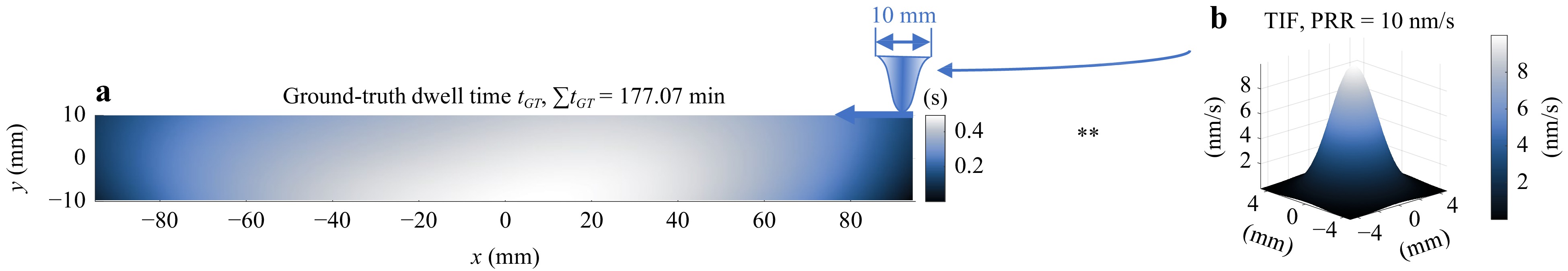
Fig. 3  The ground-truth dwell time $ t_{GT} $ a is generated by the first 144 Chebyshev polynomials. It is convoluted with a Gaussian tool influence function (TIF) b to generate the nominal removal map used in the simulation.

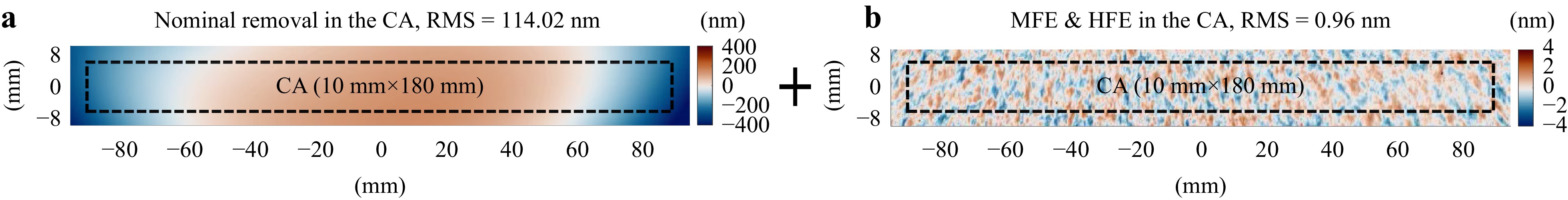
Fig. 4  The nominal target removal a generated using the dwell time and TIF shown in Fig. 3. The middle-frequency error (MFE) and high-frequency error (HFE) b are extracted from a pitch-polished mirror and added to a. The clear aperture (CA) is taken to be smaller than the outermost perimeters of the nominal target removal map by the radius of the TIF.

Secondly, we add the middle-frequency error (MFE) and high-frequency error (HFE) to the nominal target removal to simulate their influence in restoring the dwell time solution, as shown in Fig. 4b. These errors are extracted from a pitch-polished flat mirror using a high-pass Gaussian filter with a cut-off wavelength of 10 mm, equal to the TIF's diameter. These MFE and HFE thus cannot be corrected using this TIF with $ t_{GT}\left({\bf{x}}\right) $. All the dwell time optimization methods are first applied to the noise-free nominal target removal map to examine their methodological performances, then their robustness in handling MFE, HFE, and noisy data.

Lastly, to avoid the influence of edge effects⁴¹, the calculation area $ z_{e}\left({\bf{x}}\right) $ is defined to be larger than the CA by the radius of the TIF on each side of its perimeter, but only the estimated residual errors in the CA are compared. All the iterative dwell time optimization methods are kept running until the absolute root mean square (RMS) difference between the last two consecutive iterations is less than 0.01 nm. The results for each method will be demonstrated, both with and without MFE and HFE.

The additive FIM (from now on referred to as FIM) was first introduced to CCOS by Jones in 1977¹⁰, following Van Cittert’s original proposal in 1931⁶³. In FIM, as shown in Fig. 2, the initial guess to $ t\left({\bf{x}}\right) $ is taken as

where $ \alpha>0 $ is a scalar. The subsequent iterative updates of $ t\left({{\bf{x}}}\right) $ take the form of

where $ \beta>0 $ is a learning rate that controls the convergence speed and $ k\in\mathbb{Z} $. Eq. 6 indicates that the new dwell time distribution is updated using the residual between $ z_{e}\left({\bf{x}}\right) $ and the convolution of the previous dwell time and the TIF. As shown in Fig. 2, an absolute convergence is pursued in the FIM, meaning that the difference between $ t^{k+1}\left({\bf{x}}\right) $ and $ t^{k}\left({\bf{x}}\right) $ approaches zero at the convergence. However, this update rule poses several challenges in attaining this ultimate convergence.

Firstly, selecting parameters $ \alpha $ and $\, \beta $ is crucial for accuracy and convergence speed. In the conventional Van Cittert’s formula^{63, 64}, values of $ \alpha=\beta=1 $ were used in many applications like image restoration, where pixel intensity values are normalized to be within $ [0,1] $ and the actual and recovered images share the same unit. However, in CCOS, $ t\left({\bf{x}}\right) $ and $ z_{e}\left({\bf{x}}\right) $ have different units (e.g., seconds vs. nm). Therefore, using the unities for $ \alpha $ and $ \beta $ is not optimal⁶⁵. Although $ \alpha=1 $ was still used in the initial CCOS process¹⁰, it affects the dwell time accuracy and slows down the convergence rate since $ t^{0} $ may be far from the final solution. A better $ t^{0} $ in CCOS can be determined by normalizing $ z_{e}\left({\bf{x}}\right) $ by the volumetric removal rate (VRR) of the TIF $ r\left({\bf{x}}\right) $^{40, 41}, which is defined as

where $ \Omega $ is the area of the TIF. Note that in discretized implementation of Eq. 7, x is sampled in the pixel space by a measurement instrument equipped with a charge-coupled device. Therefore, VRR can be approximated by a summation of all the elements in $ r\left({\bf{x}}\right) $. The initial dwell time $ t^{0}\left({\bf{x}}\right) $ is then expressed as

where $ \alpha=1/{\rm{VRR}} $. The philosophy behind this normalization is that the $ {\rm{VRR}} $ of $ r\left({\bf{x}}\right) $ can also be written as $ \left|R\left({\boldsymbol{\omega}}={\bf{0}}\right)\right| $ where $ R\left({\boldsymbol{\omega}}\right) $ is the Fourier transform of $ r\left({\bf{x}}\right) $, which makes the use of Eq. 8 equivalent to using a normalized $ r\left({\bf{x}}\right) $ with

to generate the initial guess. Eq. 8 ensures that the volume of the deconvolved $ t^{0} $ is correct, which is critical for the convergence of the subsequent iterative refinements⁶⁴.

The convergence speed is controlled by the learning rate $ \,\beta $, also called the over-relaxation parameter^{40, 41, 65-67}, for it improves the speed of convergence of Eq. 7 if set correctly. It has been proven that the reasonable value of $ \,\beta $ ensuring the convergence is situated in the range $ (0,2] $ if the normalization in Eq. 8 is adopted^{66, 67}. Finding the optimal $\, \beta $ requires minimizing the maximum value of $ \left|1-\beta\cdot R\left({\boldsymbol{\omega}}\right)\right| $, which results in $ \,\beta=2 $ for a low-pass system with $ R\left({\boldsymbol{\omega}}\right) $ real and non-negative⁶⁷. This is the first merit of why a Gaussian $ r\left({\bf{x}}\right) $ is preferred in CCOS: the Fourier transform of a Gaussian TIF is still a Gaussian in the frequency domain. However, in actual CCOS processes, such an ideal TIF is rare, and $ R\left({\boldsymbol{\omega}}\right) $ is always complex, so finding the optimal $\, \beta $ is rather complicated. To ease the turning of $\, \beta $, an adaptive iteration scheme was proposed, in which another parameter $ \eta\in(0,1) $ was introduced to reduce $ \,\beta $⁴¹ as

when Eq. 6 begins to diverge. In detail, $ \,\beta $ is initialized with a constant in $ (0,2] $, usually with $ \,\beta=1 $ for the balance between the accuracy and convergence speed. Afterward, during the iterative refinements, the residual errors in the CA are estimated from the current and previous dwell time distributions, which are defined as $ {\rm{RMS}}_{CA}^{k+1}={\rm{RMS}}\left[z_{e}\left({\bf{x}}\right)- t^{k+1}\left({\bf{x}}\right)** r\left({\bf{x}}\right)\right]_{CA} $ and $ {\rm{RMS}}_{CA}^{k}={\rm{RMS}}\left[z_{e}\left({\bf{x}}\right)- t^{k}\left({\bf{x}}\right)** r\left({\bf{x}}\right)\right]_{CA} $, respectively, are compared. If $ {\rm{RMS}}_{CA}^{k+1}\geq{\rm{RMS}}_{CA}^{k} $, it indicates that the iterative refinement process is diverging, and Eq. 9 is executed to reduce $ \,\beta $. The iterative update is then retried with the new $ \,\beta $ until either $ {\rm{RMS}}_{CA}^{k+1}<{\rm{RMS}}_{CA}^{k} $ or a maximum number of trials is reached. As claimed in Ref. 41, this adaptive scheme eliminates the need for manual adjustment of $ \,\beta $ and automates the FIM.

The impact of $ r\left({\bf{x}}\right) $ on the convergence of FIM is also worth exploring. From the comprehensive convergence criteria related to $ r\left({\bf{x}}\right) $ derived in Ref. 64, two crucial necessary conditions (NC) can be summarized. Without loss of generality, $ {\bf{x}}={\bf{0}} $ is defined as the center of $ r\left({\bf{x}}\right) $.

The first NC of the convergence requires that $ r\left({\bf{x}}\right) $ has a solid central peak, i.e., the maximum value of $ r\left({\bf{x}}\right) $ must occur uniquely at $ {\bf{x}}={\bf{0}} $. This condition is expressed as:

The second NC demands that each even derivative of $ r\left({\bf{x}}\right) $ should have its absolute extremum at $ {\bf{x}}={\bf{0}} $, and there should be no singularities in these even derivatives, as indicated in Eq. 11:

where $ r^{(n)}\left({\bf{x}}\right) $ is the $ n $th derivative of $ r\left({\bf{x}}\right) $ for $ n=0,2,4,... $ and $ j=\sqrt{-1} $. Together, NC1 and NC2 result in the second reason why a Gaussian TIF is ideal in CCOS processes: it automatically satisfies both conditions.

A Gaussian TIF is a rotationally symmetric function with respect to the central peak, and its even derivatives are always continuous. To further illustrate this point, Fig. 5 shows the one-dimensional TIF profiles of an ideal Gaussian TIF versus other common TIFs found in CCOS processes. The bonnet⁵⁸, spin⁶⁸, and fluid-jet⁴⁹ TIFs violate NC1 since they either have a biased peak location or peaks are not unique. The spin and orbital^{68, 69} TIFs do not satisfy NC2, as their functions end abruptly, and the second derivatives are singular. The orbital TIF is also a piecewise function with discontinuous even derivatives at the transition points. All these aspects affect the convergence of the iterative routine in Eq. 6. As shown in the following sections, the other methods are derived from FIM. Therefore, the convergence analysis described above applies to those methods.

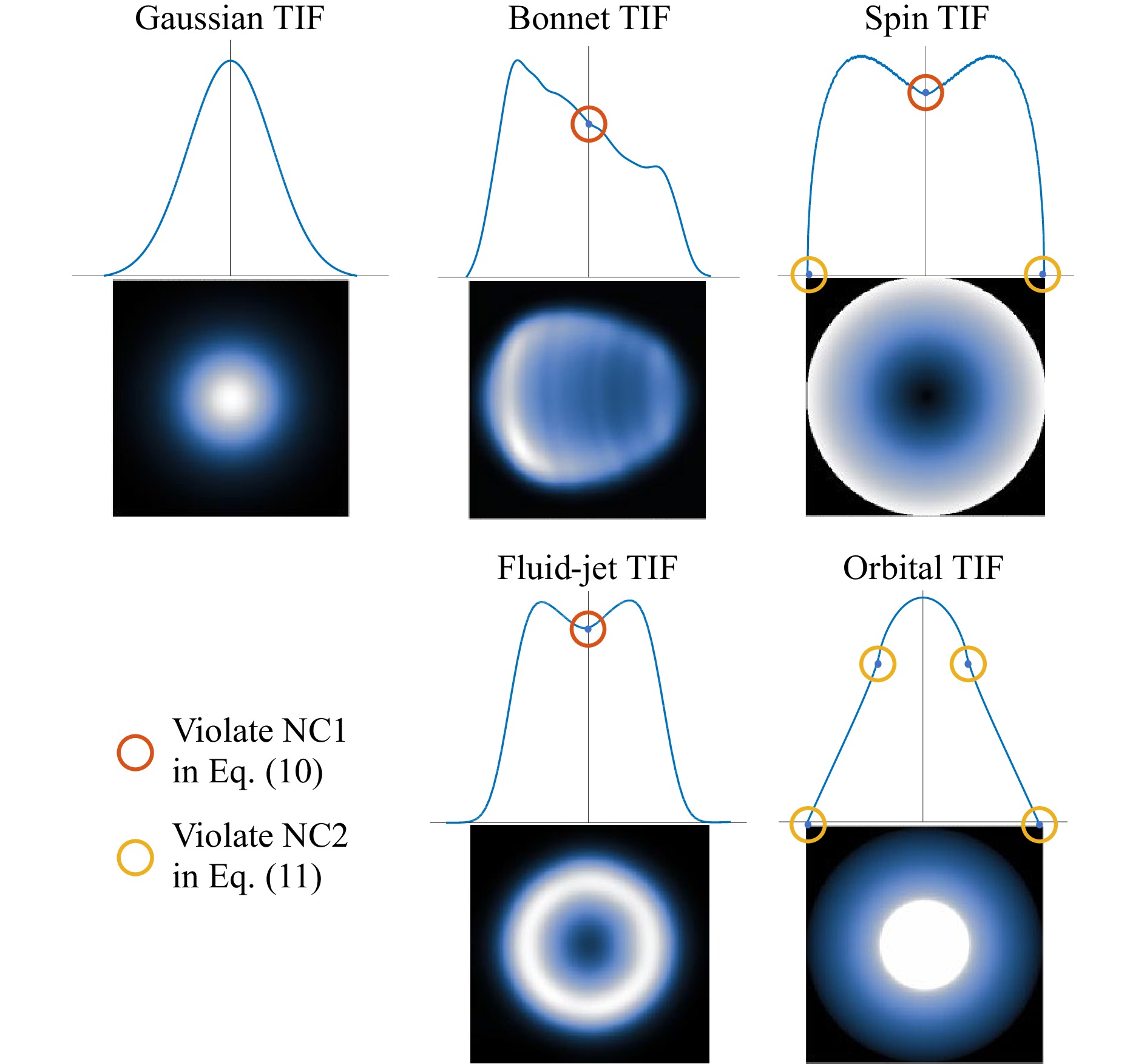
Fig. 5  One-dimensional tool influence function (TIF) profiles of the Gaussian, bonnet, spin, fluid-jet, and orbital TIFs. The points that lead to divergence are circulated.

Finally, the refinement in Eq. 6 brings edge effects to the final dwell time solution. As illustrated in Fig. 4, the convolution $ t^{k}\left({\bf{x}}\right)** r\left({\bf{x}}\right) $ is only well-defined in a region which is at least smaller than the $ z_{e}\left({\bf{x}}\right) $ by the radius of a TIF on each side of its perimeter, denoted by $ \left[z_{e}\left({\bf{x}}\right)\right]_{CA} $. Consequently, FIM yields large dwell time values along the edges of the region, which can lead to inaccurate results. If $ z_{e}\left({\bf{x}}\right) $ is defined as the entire area of the nominal removal shown in Fig. 4, the ground-truth dwell time given in Fig. 3a will not be fully recovered by FIM. To avoid this issue, it is necessary to choose a $ z_{e}\left({\bf{x}}\right) $ that is at least larger than the CA by the diameter (rather than the radius) of the TIF. If the extra area is unavailable during measurement, surface extrapolation^{32, 45, 70, 71} is necessary to generate the missing data before applying the FIM. It is worth noting that, in this study, to ensure fair comparison without edge effects, we analytically extend the nominal removal maps shown in Fig. 4 by the radius of the TIF on each side before applying FIM. The same process will be used for BAM, RIFTA and MIM. By implementing these measures, the dwell time optimization methods reviewed in this study will be more appropriately compared.

Achieving the absolute convergence of FIM in actual CCOS processes is challenging. To enhance the robustness of FIM in practice, an optimized implementation of FIM is demonstrated in Algorithm 1, which incorporates three key strategies to ensure reasonable convergence.

Firstly, the adaptive parameter tuning approach⁴¹ is adopted, wherein the learning rate $ \,\beta $ is reduced, and the update refinement is retried when the routine begins to diverge. In this study, $ \,\beta $ and $ \gamma $ are initialized to be $ \,\beta=2 $⁶⁷ and $ \eta=0.95 $⁴¹, respectively, as shown in Line 2 in Algorithm 1.

Secondly, we introduce an early stop mechanism that employs the desired error RMS $ \epsilon $ as a threshold, as shown in Line 7 of Algorithm 1. This mechanism was not mentioned in the existing FIM methods. However, in practice, it helps terminate the loop early if the current dwell time solution is already satisfactory, offering two advantages. First, it prevents the dwell time solution from deviating significantly due to the influence of noise when the number of iterations is large. This merit ensures that the result remains reasonable and is less susceptible to inaccuracies arising from noise or other sources of variation. Additionally, the early stop mechanism helps avoid unnecessary iterations, reducing the computational burden and accelerating the convergence of the optimization procedure.

Thirdly, following Ref. 41, a maximum number of iterations $ N $ is set to limit the total number of trials. If the desired error RMS cannot be achieved after $ N $ iterations, the last (and best) dwell time solution is accepted.

The FIM implementation shown in Algorithm 1 achieves improved convergence performance and robustness by implementing these three strategies. Also, the convolution in Line 5 in each iteration can be accelerated by a fast Fourier transform (FFT) so that FIM is computationally efficient and can be applied to large-scale problems in CCOS processes.

Algorithm 1 is first examined on the nominal removal shown in Fig. 4a without MFE and HFE. The resulting dwell time $ t_{FIM} $ and estimated residual height error in the CA are demonstrated in Figs. 6a, b, respectively. After 20 iterations, $ t_{FIM} $ closely replicates the shape of the nominal removal, with only 0.4% longer than the ground truth. The residual error in the CA is only 0.02 nm RMS, indicating that FIM converged to the ground-truth solution in this MFE-HFE-free case.

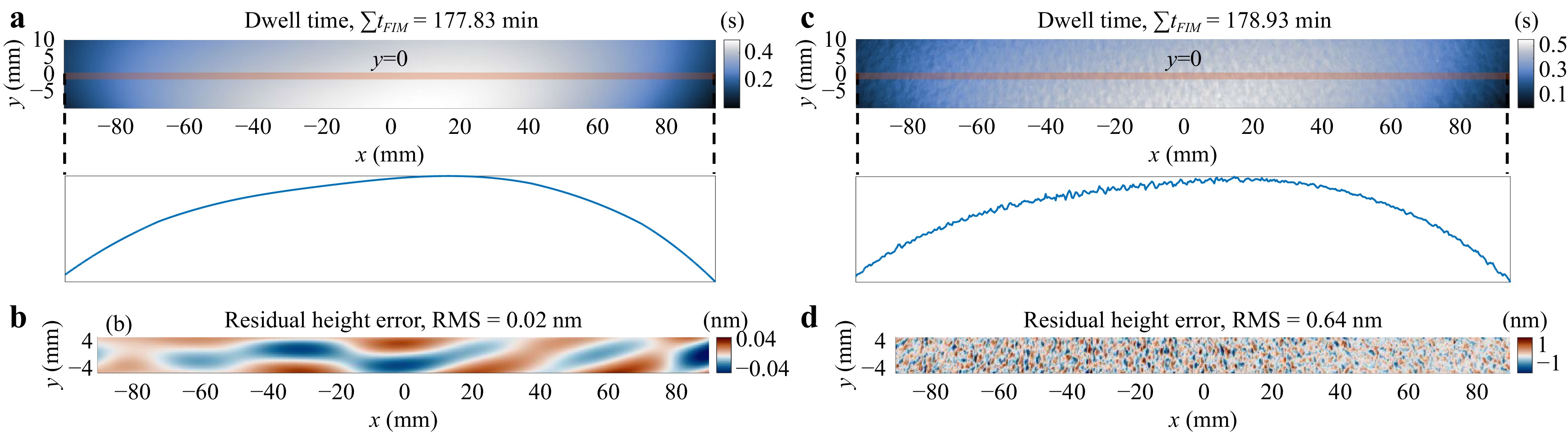
Fig. 6  Dwell time and residual height errors calculated using FIM. a, b are the dwell time and residual height errors without the middle-frequency error (MFE) and high-frequency-error (HFE), respectively. c, d are the dwell time and residual height errors with MFE and HFE, respectively. It is evident that MFE and HFE result in unsmooth dwell time.

When MFE and HFE were added, as shown in Fig. 6c, d, the calculated $ t_{FIM} $ still replicated the shape of the nominal removal and was close to the ground truth regarding the total dwell time. However, the dwell time map shown in Fig. 6c contained frequent spikes, as seen from the one-dimensional profile at $ y=0 $, which indicates that MFE and HFE lead to unsmooth dwell time. While it is possible to correct the added MFE and HFE by this dwell time to some extent, as shown in Fig. 6d, this may not be practical in actual CCOS processes since the spikes cause frequent acceleration and deceleration, which can stress the machine dynamics. A possible solution to mitigate the influence of MFE and HFE is to stop the iterative routine early once the gradients of the deconvolved dwell time exceed a certain threshold. However, determining this threshold is challenging, as it depends on the initial surface error and TIF properties. The merits of FIM are its simplicity and the well-studied convergence criteria, which lay the foundation of the other more advanced dwell time optimization methods that will be reviewed in the following sections.

We move on from FIM to BAM. As illustrated in Fig. 2, the main difference between FIM and BAM in their final formats is that a relative convergence, $ t^{k+1}/t^{k}\rightarrow1 $, is pursued in BAM instead of the absolute convergence, $ t^{k+1}-t^{k}\rightarrow0 $, in FIM. This relative convergence form results from modeling deconvolution as a Bayesian process. Specifically, in BAM, the noise is modeled as a Poisson distribution, which simplifies BAM and increases the smoothness of dwell time. The principle behind BAM and its derivation are explained in the rest of this section.

Due to the deconvolution problem's ill-posed nature, any measurement errors can be magnified and lead to undesirable results, as illustrated in Fig. 6c. To address this issue, researchers in astronomy often employ statistical estimation methods, such as BAM, for image restoration purposes^72-74. BAM, particularly the Richardson-Lucy (R-L) algorithm^{73, 74}, was introduced to solve dwell time for IBF in 2009^{28, 42}. BAM starts by defining a prior distribution $ P\left(t\right) $ over the true dwell time $ t\left({\bf{x}}\right) $, which incorporates the expected structure of the dwell time. Additionally, the probability distribution of the target removal $ z_{e}\left(x\right) $, given the true dwell time $ t\left({\bf{x}}\right) $, $ P\left(z_{e}|t\right) $, needs to be specified. Following the Bayesian paradigm, the inference towards the true $ t\left(x\right) $ should be based on $ P\left(t|z_{e}\right) $, which is defined as

where $ P\left(z_{e}\right) $ is the marginal probability of $ z_{e}\left({\bf{x}}\right) $ and can be omitted as it is independent of $ t $. Since the true dwell time $ t\left({\bf{x}}\right) $ is unknown, an estimate $ \hat{t}\left({\bf{x}}\right) $ can be obtained by maximizing the posterior probability as

which can also be expressed in the form of the minimum negative log-likelihood as

where $ L_{1}\left(t\right)=-{\rm{log}}P\left(z_{e}|t\right)-{\rm{log}}P\left(t\right) $ is the loss function, $ -{\rm{log}}P\left(z_{e}|t\right) $ is the data log-likelihood and $ -{\rm{log}}P\left(t\right) $ is a penalty term. In R-L, a non-informative prior is assumed, i.e., $ P\left(t\right)={\rm{const}} $. Therefore, the second term in Eq. 14 can be neglected. Furthermore, since most metrology instruments use charge-coupled device detectors, each component of $ P\left(z_{e}|t\right) $ is assumed to follow a Poisson distribution with the parameter $ r** t $ in R-L^{28, 42, 72}. With this assumption, a loss function $ L_{1} $ is obtained from Eq. 14 as

Since $ -{\rm{log}}\; z_{e}\left({\bf{x}}_i\right) $ is independent of $ t $, it can be eliminated from $ L_{1}\left(t\right) $ and thus, the final $ L_{1}\left(t\right) $ is written as

The optimization condition for Eq. 14 can be achieved by making the gradients of Eq. 15 equal to zero as

where $ r^{\star}\left({\bf{x}}\right)=r\left(-{\bf{x}}\right) $ is the adjoint of $ r\left({\bf{x}}\right) $. Eq. 16 can be easily fed into a gradient-descent method with $ t^{k+1}=t^{k}+\beta\cdot\nabla L_{1}\left(t\right) $, which is similar to the additive updates introduced in FIM. Nevertheless, this method generates negative values in each iteration, which should be reset to $ t_{min} $. This deviates the iteration point from the search direction given by the gradient, and convergence is not guaranteed⁷². Therefore, the R-L algorithm chose to solve this problem multiplicatively. Dividing both sides of Eq. 16 by the $ {\rm{VRR}} $ of $ r\left({\bf{x}}\right) $, it becomes

with $ (r^{\star}/{\rm{VRR}})**{\bf{1}}={\bf{1}} $ (see Eq. 7), which is also the necessary step to preserve the volume of the initial dwell time, as introduced in Section 2.1. Eq. 17 results in a multiplicative solution for the dwell time^{28, 42} as

with $ k\in\mathbb{Z} $ and $ t^{0}=z_{e} $. The merit of Eq. 18 is that the positiveness of the iterative updates is guaranteed if the initial guess $ t^{0} $ is positive, which is usually achieved by adding a constant piston term to offset $ z_{e} $.

As suggested in Refs. 28, 42, to further smooth the dwell time, a penalty term on the gradient of the dwell time was introduced as

where $ \zeta $ is a weighting parameter. Adding Eq. 19 to Eq. 14 and applying the Euler-Lagrange equation²⁸, the modified BAM iterations are deduced as

where $ \Delta $ is the Laplace operator. However, in practice, we found that $ \zeta $ is a hyperparameter that can be difficult to adjust. As claimed in Ref. 28, a small $ \zeta $ has little effect on the smoothness, while a large $ \zeta $ reduces the accuracy of the dwell time. Additionally, we found that the positivity of the dwell time in Eq. 20 cannot be automatically maintained, and the search direction of the Bayesian function is biased, leading to a lack of guarantee of convergence.

Therefore, in this study, the original R-L algorithm given in Eq. 18 is implemented in BAM. As shown in Section 2.2.2, the Poisson distribution of the likelihood is already a reasonable and smooth assumption for most optical surfaces. We recommend that if the noise level is high, this likelihood probability distribution needs to be redesigned⁷² instead of adding the penalty term given in Eq. 19.

Finally, to accelerate the convergence, we introduce the over-relaxation parameter and adaptive update strategy proposed in FIM⁴¹ to BAM, as shown in Algorithm 2, which is the same as Algorithm 1 except for Lines 1 and 5. In Algorithm 2, the two convolutions in Line 5 can be accelerated by FFT. Moreover, as the adjoint operation corresponds to the complex conjugate in the frequency domain, the FFT of r can be pre-computed. Therefore, in each iteration, only two FFTs are required, which makes BAM a computationally efficient algorithm as FIM.

We first apply Algorithm 2 to correct the nominal target removal map without MFE and HFE as shown in Fig. 4a. The optimized dwell time and the corresponding residual height error are shown in Fig. 7a, b, respectively. The dwell time map closely duplicates the shape of the nominal removal, and the total dwell time is only 0.2% longer than the ground truth. The RMS of the residual height error is 0.04 nm, which is similar to that of FIM and can be neglected. BAM does not show an obvious advantage of FIM because it essentially does the same iterative updates as the FIM but in a multiplicative manner.

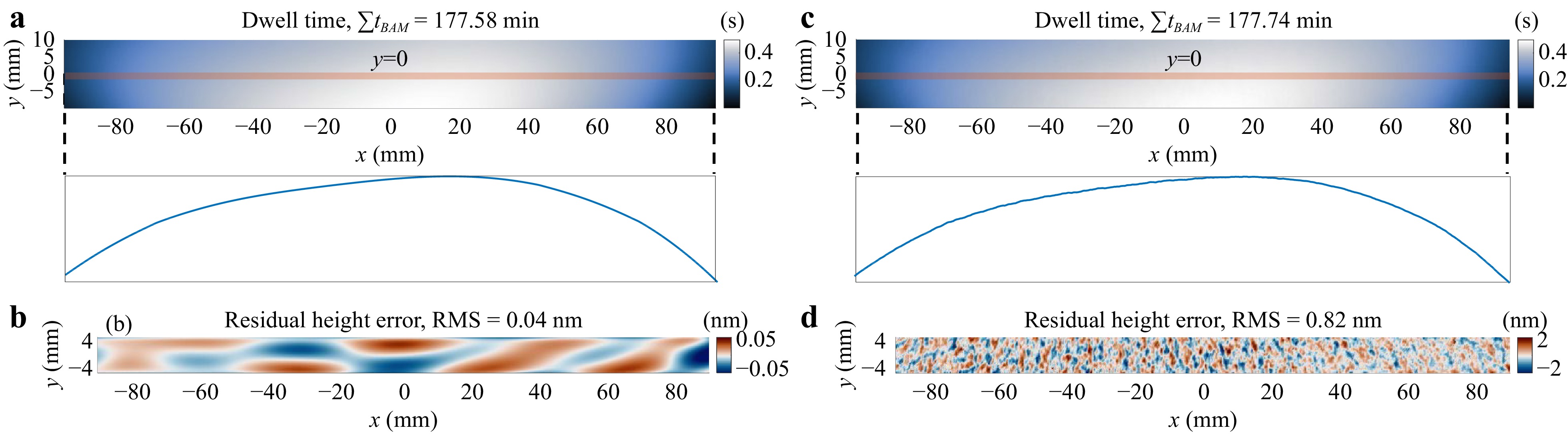
Fig. 7  Dwell time and residual height errors calculated using BAM. a, b are the dwell time and residual height errors without the middle-frequency error (MFE) and high-frequency-error (HFE), respectively. c, d are the dwell time and residual height errors with MFE and HFE, respectively. BAM handles MFE and HFE better than FIM.

We repeat the test on the nominal target removal with MFE and HFE shown in Fig. 4b. As illustrated in Fig. 7c, d, the superiority of BAM over FIM is evident in this case. The dwell time duplicates the shape of the nominal removal and is much smoother than that of FIM. The residual height error, which is 0.82 nm RMS, validates our explanation that the Poisson distribution assumption for $ P\left(z_{e}|t\right) $ is a suitable noise model, resulting in more favorable dwell time in the presence of MFE and HFE. Therefore, we encourage users to use BAM first to obtain a smooth dwell time solution and inspect the resulting residual height error. FIM can then be applied to correct this residual height error if it is still beyond the threshold $ \epsilon $, in which case the final dwell time can be obtained as $ t_{BAM}+t_{FIM} $. Although $ t_{FIM} $ may be spiky, the amplitude is small compared with that of $ t_{BAM} $, which will not significantly stress the machine dynamics in actual CCOS processes.

We have mentioned several critical convergence criteria for FIM and validated its convergence to the ground truth in the simulation. We now move one step further to pursue the analytical solution for FIM in the frequency domain when it converges, which leads to FTM.

Taking the Fourier transform of Eqs. 5 and 6 with $ \alpha=\beta=1 $ and using the convolution theorem, we have

where $ T\left({\boldsymbol{\omega}}\right) $ and $ Z_{e}\left({\boldsymbol{\omega}}\right) $ are the Fourier transforms of $ t\left({\bf{x}}\right) $ and $ z_{e}\left({\bf{x}}\right) $, respectively. Successive substitution of the iterative updates results in

in which the series in the curly brace is the first $ k+1 $ terms of the binomial expansion of $ \left\{1-\left[1-R\left({\boldsymbol{\omega}}\right)\right]\right\}^{-1} $. Therefore, $ T^{k+1}\left({\boldsymbol{\omega}}\right) $ converges to $ Z_{e}\left({\boldsymbol{\omega}}\right)/R\left({\boldsymbol{\omega}}\right) $, if $ \left|1-R\left({\boldsymbol{\omega}}\right)\right|<1 $^{64, 75}, resulting in

where $ {\cal{F}}^{-1} $ denotes inverse Fourier transform. Eq. 21 is the definition of FTM, which indicates that FIM converges to FTM when $ \left|1-R\left({\boldsymbol{\omega}}\right)\right|<1 $. Moreover, for frequencies $ {\boldsymbol{\omega}} $ at which $ R\left({\boldsymbol{\omega}}\right)=0 $, $ Z_{e}\left({\boldsymbol{\omega}}\right)=0 $ should be enforced to ensure the convergence. Hence, there is convergence from FIM to FTM if and only if

These conditions are only valid when noise is absent, which cannot be achieved in actual CCOS processes. With the presence of noise, when the amplitude of $ R\left({\boldsymbol{\omega}}\right) $ at specific frequencies are close to zero, any noise in $ Z_{e}\left({\boldsymbol{\omega}}\right) $ at those frequencies will be amplified, resulting in an inaccurate dwell time solution^{28, 44}.

To address this issue, a thresholded inverse filter $ \bar{R}\left({\boldsymbol{\omega}};\gamma\right) $ has been introduced in place of $ R\left({\boldsymbol{\omega}}\right) $ in Eq. 21, given by

where $ \bar{R}\left({\boldsymbol{\omega}};\gamma\right) $ is defined as

The parameter $ \gamma $ is the threshold for constraining the inverse of $ R\left({\boldsymbol{\omega}}\right) $^{20, 38}.

It is worth noting that, however, determining the optimal value for $ \gamma $ is nontrivial and depends on the noise level in the surface error map and TIF properties. Therefore, FTM is hard to apply in practice, leading to the development of RIFTA. RIFTA effectively addresses the $ \gamma $ tuning problem through an optimization approach. The optimization algorithm in RIFTA plays a crucial role in enabling FTM to function correctly. Therefore, in the subsequent sections, we focus on elaborating on the principle of RIFTA and only provide its performance evaluation.

The optimal threshold $ \hat{\gamma} $ in FTM is found by RIFTA through minimizing the estimated residual error in the CA, expressed as

It is worth noting that Eq. 23 is non-linear and not continuous due to the thresholding operations involved in the calculation of $ \bar{R}\left({\boldsymbol{\omega}};\gamma\right) $. As a result, any derivative-based optimization algorithm will struggle to solve this optimization problem. Therefore, RIFTA utilizes derivative-free optimization methods, such as the Nelder-Mead⁷⁶ or pattern search (PS) algorithm⁷⁷. These methods are particularly effective when the number of variables is small and the computational complexity of the loss function is low⁷⁸. Since $ \gamma $ is the only variable to be optimized and the evaluation of Eq. 23 can be accelerated by FFT, derivative-free optimization methods are thus suitable for finding $ \hat{\gamma} $.

RIFTA also innovates an iterative scheme to minimize the total dwell time. As illustrated in Figs. 3 and 4, the area $ z_{e} $ used for calculating the dwell time is larger than the required CA. To ensure that the dwell time is positive, $ z_{e} $ needs to be at least offset by a piston equal to the magnitude of its smallest entry. Nevertheless, if the smallest entry is located outside the CA, this piston adjustment may lead to an unnecessary increase in total dwell time. To address this issue, RIFTA iteratively adds pistons to $ z_{e} $ based on the previous residual errors in the CA, which can be expressed as

These iterations are performed until the RMS difference between the current and previous residual errors in the CA is less than a certain threshold or the maximum number of iterations is reached. With this iterative scheme, RIFTA ensures that $ z_{e} $ is adjusted by the smallest (i.e., optimal) piston, eliminating unnecessary dwell time increment.

In most CCOS processes, we are only interested in the form error correction, in which only the relatively low-frequency error (LFE) determined by the machine tool’s removal capability are corrected, with the MFE and HFE components left on the optical surface, which will then be corrected using either a smaller machine tool or a smoothing process. With the assumption of LFE correction, as shown in Fig. 2, RIFTA can be simplified by removing the thresholded inverse filtering and directly using the entire frequency components of the target removal $ z_{e} $. Therefore, in this study, we further simplify the implementation of RIFTA by approximating $ \bar{R}\left({\boldsymbol{\omega}};\gamma\right)^{-1} $ with $ \gamma $ as

where $ \gamma $ becomes the optimal multiplier such that

and the final dwell time is obtained as

It is worth mentioning that the dwell time obtained in Eq. 27 is equivalent to finding the optimal initial guess for FIM defined in Eq. 5 that minimizes the estimated residual error in the CA. Although the dwell time solution contains the same frequency components as the target removal, as will be shown in Section 2.3.3, this is always a suitable assumption for CCOS applications, as it guarantees that no new MFE or HFE will be introduced to the dwell time solution, thus adding implicit smoothness constraints. Combined with the total dwell time reduction scheme, the optimized implementation of RIFTA is illustrated in Algorithm 3.

As shown in Line 2, the initial guess of $ \gamma $ for the first iteration is taken as the amplitude of the direct current component of $ R\left({\boldsymbol{\omega}}\right) $, which is $ \gamma^{0}=\left|R\left({\boldsymbol{\omega}}={\bf{0}}\right)\right| $, as it is close to the optimal value⁶⁶. Also, it is essential to note that $ \gamma $ is optimized in each iteration, as the target removal $ z_{e} $ is continuously adjusted to minimize the total dwell time. The iterative reduction of the dwell time is stopped when the desired residual error is attained, or the current residual error in the CA stops decreasing, indicating divergence.

We apply RIFTA in Algorithm 3 to the nominal removal in Fig. 4a without MFE and HFE components. Fig. 8a, b show the optimized dwell time and the corresponding residual height error map, respectively. Thanks to the iterative dwell time reduction scheme with respect to the CA, RIFTA achieves a total dwell time of 129.28 min, which is about 50 min shorter than the ground truth, FIM, and BAM. This can be visually observed by the smaller dwell time entries along the edges of the dwell time map in Fig. 8a. However, the residual height error, 0.19 nm RMS, as illustrated by Fig. 8b, is slightly larger than those of FIM and BAM, indicating that RIFTA is methodologically less accurate than FIM and BAM, as it includes a more strict smoothness constraint defined in Eq. 27.

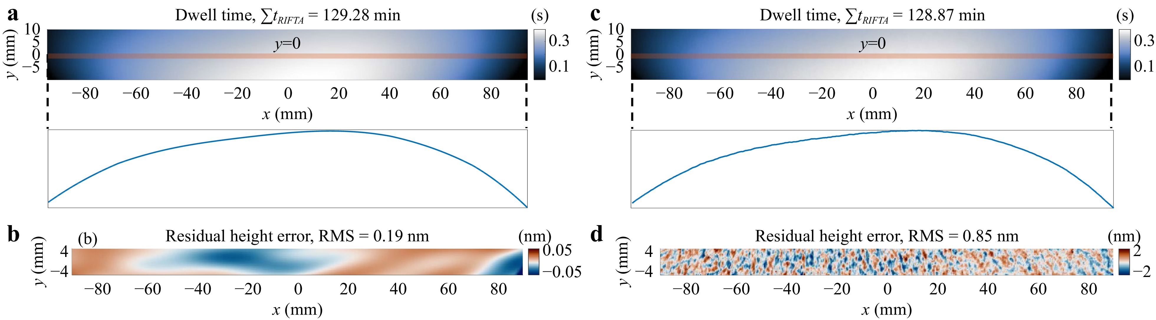
Fig. 8  Dwell time and residual height errors calculated using RIFTA. a, b are the dwell time and residual height errors without the middle-frequency error (MFE) and high-frequency-error (HFE), respectively. c, d are the dwell time and residual height errors with MFE and HFE, respectively. RIFTA not only handles MFE and HFE well, but also has shorter total dwell time than FIM and BAM.

When MFE and HFE are present, as shown in Fig. 8c, d, the two advantages of RIFTA over FIM and BAM become evident. First, RIFTA achieves a much smoother dwell time than FIM, resulting in the same residual error level as BAM. Second, this residual error is obtained with a 27% shorter total dwell time. This total dwell time reduction scheme is especially significant in large optics fabrication, where such a percentage means efficiency improvements of days or even months. Hence, we recommend always using RIFTA to solve the function-form dwell time optimization problem if there is enough measurement data outside the CA, as it handles MFE and HFE well while minimizing the total dwell time. In most cases, this RIFTA solution is satisfactory. However, if the desired residual error threshold is not achieved, FIM can be further applied to the residual error map, and the final dwell time is obtained as $ t_{RIFTA}+t_{FIM} $.

In the previous sections, we assumed that the data outside the CA is always available for optimizing the dwell time. Consequently, the dwell time solution is always satisfactory, and the residual error in the CA is small. However, there are cases when only the data inside the CA is available for dwell time optimization, which typically happens when the desired residual error is not attained after one CCOS process. For instance, Fig. 9 shows the interferometric measurement of an elliptical-cylindrical surface after one IBF process. It is evident from the reconstructed height map that the errors along the edge of $ z_{e} $ is large, which is resulted from the insufficient boundary dwell time during the dwell time optimization. Suppose the desired residual error in the CA is not achieved, and no smaller TIF is available. In that case, the dwell time solution for the next IBF run will be inaccurate since it will consume much dwell time to correct the significant boundary errors, which is unnecessary.

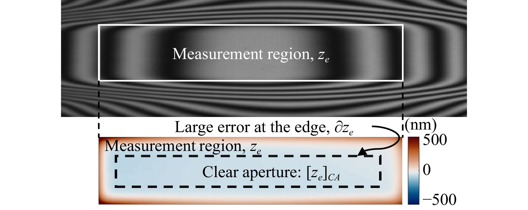
Fig. 9  The large edge errors in $ z_{e} $ will resulted from the last IBF process due to insufficient boundary dwell time.

To address this issue, a more proper way to calculate the dwell time is to rely on surface extrapolation to obtain the extra data in $ z_{e} $, using only the measurements within the CA. Conventional surface extrapolation methods include the Papoulis-Gerchberg extrapolation^{20, 70, 79, 80}, nearest-neighbors extrapolation^{70, 81}, Gaussian extrapolation^{70, 81}, and natural neighbor extrapolation (NNE)⁸¹. A descending profile has even been proposed to reduce the extended errors along the boundary and help decrease the total dwell time⁸¹. However, despite the widespread adoption of these surface extrapolation methods in CCOS processes, two challenges remain that restrict their ability to achieve accurate dwell time solutions.

First, the measured errors in the CA are not adequately modeled so that the continuity along the extrapolation boundary is not guaranteed, especially when the error in the CA is anisotropic.

Second, MFE and HFE that a particular TIF cannot correct are also extrapolated. This improper handling of extrapolation results in unsatisfactory boundary data in $ z_{e} $ and expected errors in the unreliable dwell time solution.

Polynomial-based extension. To answer these two challenges, RISE was proposed⁴⁵. Firstly, RISE models the errors in the CA using orthogonal polynomials, which eliminates the continuity issues at the boundaries of the CA. We define a boundary condition on $ z_{e} $ as its outermost perimeter, denoted as $ \partial z_{e} $. In the fitting process, besides the known error in the CA, $ \left[z_{e}\right]_{CA} $, a boundary $ \partial z_{e} $ is also included to tune the fitting coefficients and the extrapolated data. The simplest way is to set $ \partial z_{e}=0 $. However, this is so strict that it may cause significant errors in the dwell time. Instead, $ \partial z_{e} $ can be initialized as the boundary of $ \left[z_{e}\right]_{CA} $ after NNE, which is denoted by $ z_{e|NNE} $, i.e., $ \partial z_{e}=\partial z_{e|NNE} $, since NNE guarantees the $ C^{1} $ continuity along the extrapolation boundary⁸¹. Nevertheless, as NNE amplifies the errors along the CA boundary and may bring unnecessary dwell time, RISE introduces a factor $ \xi,\; \xi\in(0,1] $, which is multiplied to $ \partial z_{e|NNE} $ to flexibly adjust the figure errors in the extrapolation region and tune the dwell time. Based on the above description, the polynomial-based extension in RISE, denoted as $ z_{e|Poly}\left({\bf{x}}_i\right) $, can be summarized as the following constrained least-squares problem

where $ c_{j} $ is the coefficient of the $ j $th polynomial $ Q_{j} $. The extrapolated surface is obtained as $ z_{e|Poly}\left({\bf{x}}_i\right)=\sum_{j}\hat{c}_{j}Q_{j} $, after which the dwell time $ t $ is optimized using RIFTA introduced in Algorithm 3.

Iterative refinement of the dwell time. Even with the proposed polynomial-based extension, the obtained dwell time may remain sub-optimal due to the possible errors introduced during the extrapolation and the unreliable, ill-posed deconvolution. Therefore, a refinement of dwell time is performed by iteratively extrapolating the residual error in the CA to approach a better dwell time solution progressively. Denoting the residual error in the CA in the $ (k+1) $th $ (k\geq0) $ iteration as $ e_{CA}^{k+1}=z_{e}-\left[r**t\right]^{k} $, the polynomial extension is applied to $ e_{CA}^{k+1} $ to obtain $ z_{e|Poly}^{k+1} $. The resulting incremental dwell time $ \Delta t $ obtained using RIFTA is then added to the updated dwell time solution $ t^{k+1} $ as

where $ h $ is the learning rate that controls the convergence speed. Additionally, to eliminate the unnecessary dwell time added in $ \Delta t $ in each iteration, an intelligent piston adjustment⁴⁵ is performed on $ z_{e|Poly}^{k+1} $ and only the resulted $ \Delta z_{e|Poly}^{k+1} $ is used with RIFTA to obtain $ \Delta t $ and updates $ t^{k+1} $ as

where

This piston adjustment eliminates the extra removal added during each iteration and hence relaxes the positivity requirement of $ \Delta t $ but only guarantees the final $ t^{k+1} $ to be positive.

Algorithm 4 illustrates the implementation of RISE based on RIFTA (see Algorithm 3) and the iterative polynomial-based surface extrapolation. In this study, the polynomial order M is selected as 144, the same as the generated ground-truth dwell time shown in Fig. 3a for comparison among different methods. In practice, the residual error between $ \left[z_{e}\right]_{CA} $ and $ \left[z_{e|Poly}^{0}\right]_{CA} $ can guide the selection of appropriate polynomial orders⁴⁵. One candidate threshold for the RMS of the residual error can be selected as the random errors of the measurement instruments employed in the CCOS process. Additionally, the learning rate $ h=0.5 \sim 0.8 $ is a proper range that allows RISE to converge in less than ten iterations⁴⁵, and in this study, $ h=0.5 $ is used, as shown in Line 2. Finally, the multiplier $ \xi $ is set to 1 for the boundary condition defined in Eq. 28, as we prioritize accuracy in the comparison.

Fig. 10a, b demonstrate the dwell time and estimated residual error after applying Algorithm 4 to the nominal removal in Fig. 4a without MFE and HFE, respectively. While RISE achieves the same residual error level in the CA as RIFTA, the edge errors are more prominent than RIFTA, and a longer total dwell time is required, resulting from the iterative, polynomial-based extension strategy.

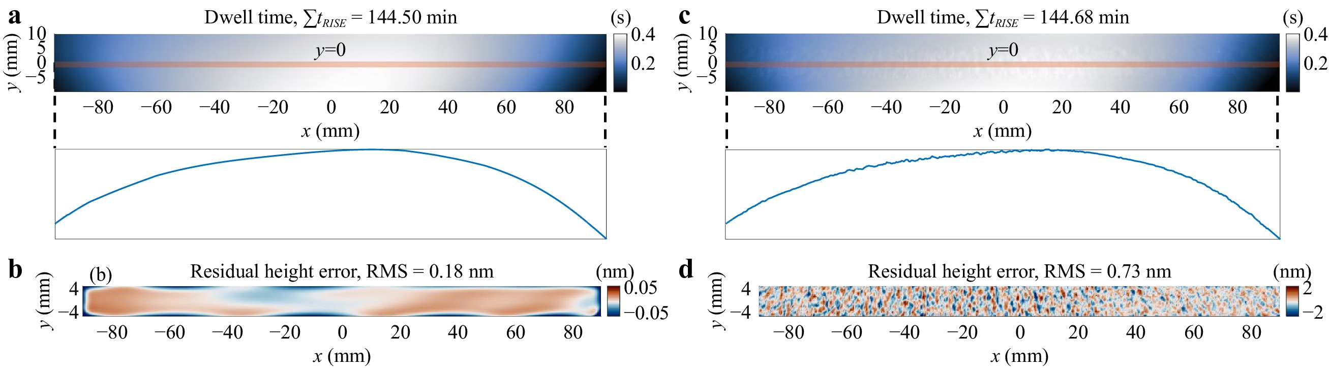
Fig. 10  Dwell time and residual height errors calculated using RISE. a, b are the dwell time and residual height errors without the middle-frequency error (MFE) and high-frequency-error (HFE), respectively. c, d are the dwell time and residual height errors with MFE and HFE, respectively. RISE has larger edge residual errors and longer total dwell time than those of RIFTA, but it only uses the measurements in the clear aperture.

We then test the nominal removal with the addition of MFE and HFE given in Fig. 4b. The results are given in Fig. 10c, d, respectively. While the obtained total dwell time is similar to that of the MFE-HFE-free case and a lower residual error RMS is attained compared to RIFTA, the smoothness of the dwell time is degraded in RISE, which exposes another effect of the polynomial-based extension in RISE, that the smoothness of the dwell time may be affected if the polynomial orders are not well selected.

To obtain smoother dwell time solutions, smaller numbers of polynomial orders can be attempted using the thresholding method introduced in Section 2.3.1. Also, to reduce the total dwell time, a smaller $ \xi $ can be employed in restricting the amplitude of the boundary conditions. Since RISE adopts RIFTA, a very computationally efficient method, multiple trials with different values of the polynomial orders and $ \xi $ can be conducted to balance the total dwell time and the residual error in the CA.

We have introduced four function-form methods in this section. As shown in Fig. 2, FIM applies the additive Van Cittert’s iterations to converge to the optimal dwell time solution progressively. Similarly, BAM uses the multiplicative, R-L algorithm to obtain a smooth dwell time solution with the assumption of a Poisson distribution of the noise model. While FIM pursues absolute convergence, BAM minimizes the relative difference between consecutive iterations. With the absence of noise, FIM converges to FTM. However, to handle the noisy CCOS processes, a threshold is required to restrict the noisy frequencies in FTM, leading to the development of RIFTA, which finds the optimal threshold for FTM while minimizing the total dwell time through an iterative piston adjustment scheme. RIFTA, if we assume that only low-frequency components are corrected in a CCOS process, is equivalent to finding the best initial guess for FIM, which further simplifies RIFTA. RISE improves upon RIFTA by using a polynomial-based surface extrapolation method to optimize dwell time when only data in the CA is available and iteratively refine the dwell time solution. RIFTA and RISE achieve comparable accuracy and smoothness to the state-of-the-art methods with significantly reduced total dwell time. Therefore, we recommend the users use RIFTA and RISE in function-form dwell time optimization problems for CCOS processes.

This section will discuss the matrix-form methods for dwell time optimization in depth. These methods are based on the linear system given in Eq. 4. The main challenge with this method is that the matrix $ {\bf{R}} $ is always near singular, making it hard to obtain a stable solution. The most important merit of the matrix-form method is that it enables arbitrary dwell positions, meaning that the dwell points $ {\bf{u}}_i $ and surface points $ {\bf{x}}_j $ can be different, i.e., $ {\bf{u}}_i\neq {\bf{x}}_j $ in Eq. 3. This adds flexibility when more complex tool paths are needed to restrain MFE³⁴ or fabricate free-form optics. In this section, we will review the matrix-form dwell time optimization methods that can obtain reasonable dwell time solutions.

Analogous to Eq. 6, Van Cittert’s iterations can be performed in discrete matrix form^{49, 66} as

In fact, FIM is a special case of MIM, in which $ {\bf{R}} $ is a square matrix. The NC1, given in Eq. 10, can be represented in matrix form⁶⁶ as

Like FIM,when NC1 and NC2 hold, there is a convergence criterion in MIM related to the learning rate $ \beta $ determined from the matrix $ {\bf{R}} $. First, it has been found that if $ {\bf{R}} $ is a positive definite matrix, the convergence interval for $ {\bf{R}} $ is

where $ \lambda_{{\bf{R}}}^{max} $ is the largest eigenvalue of $ {\bf{R}} $⁶⁶. However, as $ {\bf{R}} $ is always near singular, we need to multiply $ {\bf{R}} $ by its transpose, and hence $ {\bf{R}}^{{\rm{T}}}{\bf{R}} $ becomes positive definite. By multiplying the two sides of Eq. 3 with $ {\bf{R}}^{{\rm{T}}} $, we obtain

for which the iterative form of Eq. 32 becomes

Therefore, the range of $ \beta $ can be determined by finding the maximum eigenvalue $ \lambda_{{\bf{R}}^{{\rm{T}}}{\bf{R}}}^{max} $ of $ {\bf{R}}^{{\rm{T}}}{\bf{R}} $. Indeed, an estimate of the maximum eigenvalue is sufficient for MIM. As illustrated in Ref. 35, the estimated range for $\, \beta $ is approximated as

It is worth mentioning that multiplying by $ {\bf{R}}^{{\rm{T}}} $ not only simplifies the determination of the learning rate but also brings two benefits. First, it enables MIM to be used even when the dwell points $ {\bf{u}}_{i} $ and surface points $ {\bf{x}}_{j} $ are with different sampling positions. The operation of $ {\bf{R}}^{{\rm{T}}}{\bf{z}}_{e} $ projects $ {\bf{z}}_{e} $ to the same space as $ {\bf{t}} $. More importantly, multiplying by $ {\bf{R}}^{{\rm{T}}} $ acts as a low-pass pre-filtering process. In each iteration, $ t^{k+1} $ is updated by the filtered residual, $ {\bf{R}}^{{\rm{T}}}\left({\bf{z}}_{e}-{\bf{R}}{\bf{t}}^{k}\right) $. As demonstrated in Section 3.1.2, this pre-filtering operation helps smooth the dwell time solution.

Algorithm 5 shows the implementation of MIM, which is very similar to that of FIM. Both methods can use the adaptive learning rate⁴¹ and early stop strategies. The maximum value in Eq. 35 initializes the learning rate $ \,\beta $ in Line 2. If the iteration becomes divergent, $\, \beta $ will be reduced in Line 16 and the iteration is retried. The initial guess for the dwell time in MIM, as shown in Line 3, is given as

where $ \alpha=1/{\rm{VRR}} $. It is worth noting that the most time- and memory-consuming operation in Algorithm 5 is the construction of the convolution matrix $ {\bf{R}} $ when the size of the optical surface is large, and the dwell points are dense. However, since $ {\bf{R}} $ is sparse, with all non-zero elements concentrating along its diagonals, storing $ {\bf{R}} $ using sparse matrix structures, such as compressed-row or compressed-column format is always recommended. The subsequent operations on $ {\bf{R}} $ involve sparse matrix arithmetic, which have been well accelerated by math libraries on modern computing hardware.

We applied MIM on the simulation data given in Fig. 4, and the results are shown in Fig. 11. In the case without MFE and HFE shown in Fig. 11a, b, compared to FIM, the total dwell time is about 1-min longer while the residual height error RMS is slightly larger. This negligible reduction in accuracy resulted from the introduction of $ {\bf{R}}^{{\rm{T}}} $ for pre-filtering.

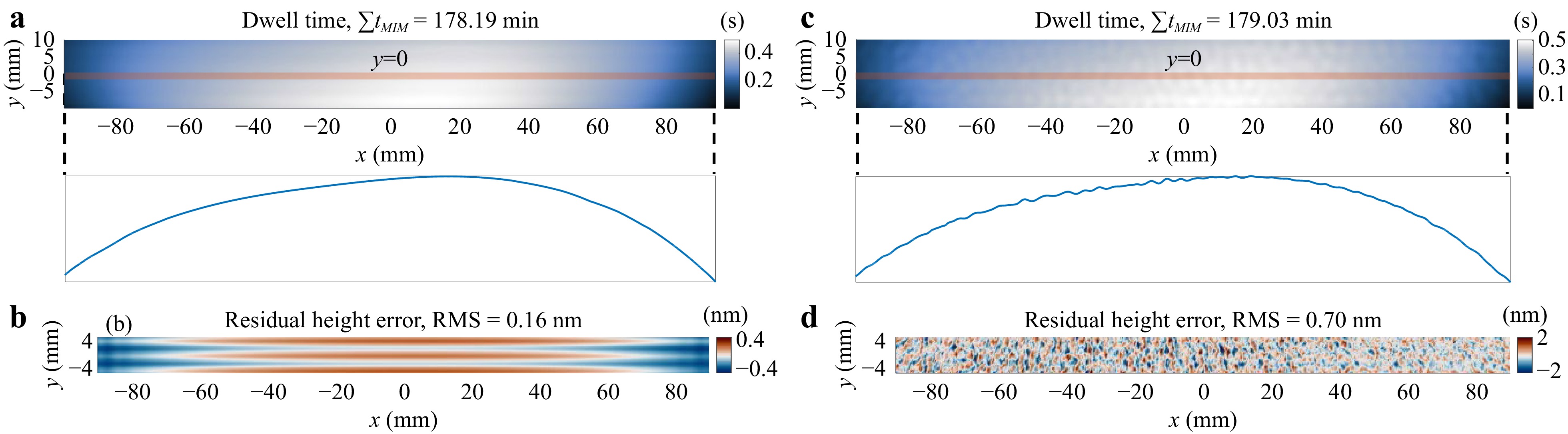
Fig. 11  Dwell time and residual height errors calculated using MIM. a, b are the dwell time and residual height errors without the middle-frequency error (MFE) and high-frequency-error (HFE), respectively. c, d are the dwell time and residual height errors with MFE and HFE, respectively. It is evident that prefiltering with $ {\bf{R}}^{{\rm{T}}} $ smooths the dwell time.

On the other hand, in the case of MFE and HFE shown in Fig. 4c, d, the merit of multiplying with $ {\bf{R}}^{{\rm{T}}} $ is evident. With a slight degradation of algorithmic accuracy, the dwell time profile is much smoother than that obtained from FIM shown in Fig. 6c, indicating that the dwell time optimization is unaffected by MFE and HFE in MIM. Therefore, we recommend that users always use MIM with $ {\bf{R}}^{{\rm{T}}} $ pre-filtering to obtain more reliable dwell time solutions.

Moreover, as FIM is a special case of MIM, this pre-filtering idea in MIM can also be introduced to FIM as

if the smoothness of the dwell time solution optimized with the conventional FIM is unsatisfactory and the small influence on the residual error is acceptable.

Instead of solving the matrix-form equation (see Eq. 4) iteratively using MIM, it can also be solved directly with the least-squares method. However, as the least-squares solution to Eq. 4 is known to be unstable, the Tikhonov regularization has been introduced to obtain a reasonable dwell time solution. With the Tikhonov regularization, the solution to Eq. 4 can be obtained by optimizing the following equation⁵⁷

where $ \rho $ is a damping factor that penalizes the magnitude of the solution vector. This section will demonstrate how Tikhonov regularization helps stabilize the solution and improve the overall performance.

The Tikhonov-regularized solution to Eq. 37 is equivalent to finding the particular least-squares solution, which is the minimum in the $ l_{1} $-norm sense⁵⁷ expressed as

SVD can be used to find the solution of $ {\bf{t}} $ in this sense as

where $ \sigma_{i} $, $ i=0,1,2,\ldots,M-1 $, are the singular values appearing in non-increasing order; $ {\bf{u}}_i $ and $ {\bf{v}}_i $ are the left and right singular vectors of $ {\bf{R}} $, respectively. As many of the singular values are close to zero since $ {\bf{R}} $ is nearly singular, TSVD should be used instead of SVD⁵⁴, in which only the first $ K $ singular values are kept as

There are two difficulties in solving for $ {\bf{t}} $ directly using Eq. 40 in practice. First, the total dwell time is not guaranteed to be minimal, even though $ |{\bf{t}}|_{1} $ is minimized, since the positivity of $ {\bf{t}} $ cannot be ensured in Eq. 40. To mitigate the negative entries in $ {\bf{t}} $, multiple trials of extra piston adjustments of $ {\bf{z}}_{e} $ are necessary. Additionally, determining the optimal number of singular values $ K $ is difficult. While the “L” curve approach has been attempted⁵⁴, in which $ K $ at the turning point on the curve was selected, the computation of SVD is extremely time-consuming, making it impractical to generate sufficient data points for plotting the “L” curve.

To address the two difficulties associated with TSVD, an efficient iterative solver names LSQR⁸² has been proposed, taking advantage of the sparse nature of $ {\bf{R}} $. Instead of directly calculating all the singular values, the LSQR algorithm employs iterative steps to refine the dwell time solution. It gradually converges to a solution that balances the minimization of the residual error and the regularization imposed by TSVD^{16, 29, 30, 50-52, 56, 57}. The final solution to Eq. 37 is closely related to the minimum $ l_{1} $-norm solution given by Eq. 39 as

When $ \rho=0 $, Eq. 41 is equivalent to Eq. 39. The $ \rho^{2} $ term in the denominator “damped” the least-squares solution by preventing small values of $ \sigma_{i} $ from causing the solution $ {\bf{t}} $ to grow excessively large. The parameter $ \rho $ plays a crucial role in balancing the smoothness, accuracy, and distribution of negative entries in $ {\bf{t}} $⁵³. The choice of $\, \rho $ impacts the characteristics of the solution. Larger values of $\, \rho $ tend to result in a smoother dwell time profile with fewer negative entries, but at the cost of reduced accuracy. Conversely, smaller values of $ \,\rho $ can lead to increased accuracy but may result in a less smooth dwell time profile and potentially more negative entries in $ {\bf{t}} $^{53, 57}.

Therefore, finding an appropriate value for $ \rho $ is a trade-off between achieving the desired level of smoothness, accuracy and minimizing negative entries in $ {\bf{t}} $. Traditionally, the selection of a proper damping factor $ \rho $ has been based on trial-and-error^{53, 57} or the “L” curve obtained by time-consuming exhaustive search⁵⁴, which can be time-consuming. Researchers have also explored finding a typical range for $ \rho $ based on the PRR of a TIF, which provides some guidance for choosing $ \rho $⁵². However, this range is unstable when the desired residual error is small. Due to the sensitivity of the damping factor, it is essential to carefully and automatically evaluate and choose the optimal $ \rho $ based on specific criteria. The derivative-free optimization method used in RIFTA and RISE reviewed above can be employed to automate the determination of the optimal $ \rho $ in this problem⁵⁸, which will be detailed in the following section.

The optimized implementation of LSQR is shown in Algorithm 6, which automates the damping factor tuning while maintaining the positiveness of the dwell time solution⁵⁸.

The automatic $ \rho $ optimization algorithm uses the merit criterion of the residual error RMS, as indicated in Lines 6 − 8. The positivity in the evaluation of $ {\bf{t}} $ is ensured through Line 11, where $ {\bf{t}} $ is adjusted such that its smallest value $ {\rm{min}}({\bf{t}}) $. Calculating the derivatives of the merit function is challenging, making it necessary to employ derivative-free optimization methods as introduced in Section 2.3.1 are used. The PS optimization method^{58, 77} is selected in this study, as shown in Line 3. It is worth mentioning that the iterative Least-squares with MR factorization (LSMR) solver is utilized to calculate $ {\bf{t}} $ instead of LSQR, as shown in Line 10 because it converges faster for incompatible linear systems (i.e., the dwell points are less than the sampling points of a measured workpiece surface) and is more computationally efficient^{58, 83}.

For PS to converge faster, a suitable initial guess for $ \,\rho $, denoted as $ \,\rho_{ini} $, is required. While $\, \rho_{ini} $ can be selected as a value suggested in Ref. 29 or randomly picked from the typical range⁵², it has been observed that these values may not be appropriate for the positiveness adjustment. Instead, as depicted in Line 2, a more reliable derivative-free optimization method, Particle Swarm Optimization (PSO), is utilized to generate a well-suited $\, \rho_{ini} $, eliminating the need for manually determining an initial guess⁵⁸. To mitigate the computational burden of PSO, the algorithm is stopped early when it stalls at a merit function value. Ultimately, the calculation of $ {\bf{t}} $ involves utilizing the optimized damping factor $ \hat{\rho} $ obtained from PS in Line 4.

We apply Algorithm 6 to optimize dwell time for the nominal removal maps with and without MFE and HFE. The results are presented in Fig. 12. As shown in Fig. 12a, c, both dwell time maps closely resemble the ground truth, and the smoothness of the dwell time profile is not affected much by MFE and HFE thanks to the damping factor optimization method.

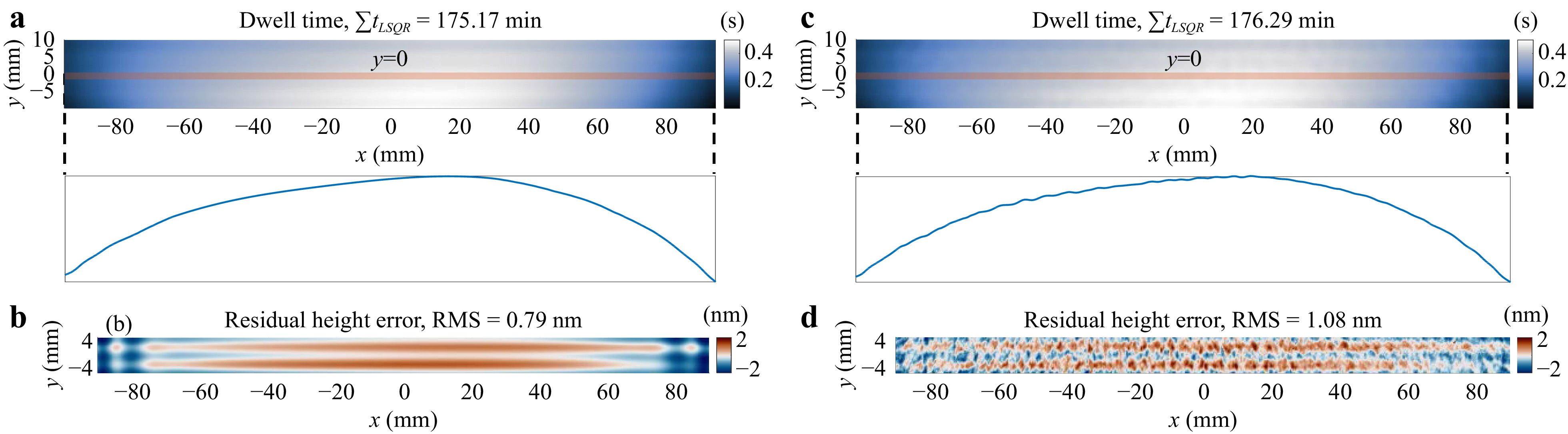
Fig. 12  Dwell time and residual height errors calculated using LSQR. a, b are the dwell time and residual height errors without the middle-frequency error (MFE) and high-frequency-error (HFE), respectively. c, d are the dwell time and residual height errors with MFE and HFE, respectively.

However, as depicted in Fig. 12b, d, the accuracy of LSQR is lower than those obtained from MIM. Notably, both residual error maps exhibit LFE components that could have been corrected, indicating that more iterations may be required for LSQR to achieve the same level of accuracy as MIM. Thus, we recommend that users relax the constraint of the maximum number of iterations and mainly rely on the residual error RMS to stop the LSQR method.

In the Tikhonov-regularized method, the damping factor is added to penalize the significant variations in the dwell time solution, improving the smoothness and reducing the number of negative entries⁵⁷. Alternatively, these objectives can be achieved by solving Eq. 4 with the CLLS algorithm^{30, 60, 59, 84}, which incorporates appropriate constraints to limit the search space of the dwell time solution. The CLLS problem can be formulated as

where $ t_{min}\leq {\bf{t}}\leq t_{max} $ is the bounding constraints that ensure the positivity of $ {\bf{t}} $⁵⁹ and can be tuned based on the constraints of the machine dynamics³⁰; $ {\bf{A}} $ is the adjacency matrix of $ {\bf{t}} $ and $ {\bf{b}} $ is the upper limit of the absolute difference between every two adjacent elements in $ {\bf{t}} $^{59, 84}. Therefore, the inequality constraints can impose smoothness constraints on the dwell time solution. To solve Eq. 42, it can be reformulated as a general quadratic programming problem by letting $ {\bf{H}}={\bf{R}}^{{\rm{T}}}{\bf{R}} $ and $ {\bf{q}}=-{\bf{R}}^{{\rm{T}}}{\bf{z}}_e $, resulting in

and any quadratic programming method (e.g., the active-set method in Ref. 59) can be employed to solve this problem.

It can be observed from Eq. 42 that setting proper values for the dwell time difference constraints in the vector $ {\bf{b}} $ is a non-trivial task. Direct utilization of the CLLS algorithm may lead to inaccurate dwell time solutions, especially when the constraints in $ {\bf{b}} $ are too strict while the local shape changes in the target removal $ {\bf{z}}_e $ are large. To answer this challenge, the optimized implementation of CLLS, employing the coarse-to-file scheme⁵⁹, is presented in Algorithm 7.

On the coarse level, as shown in Lines 3 and 4, the inequality constraints in Eq. 42 are disabled, and an initial dwell time solution $ {\bf{t}}_{ini} $ is calculated as

which is not always smooth enough. Therefore, a polynomial fitting is performed on $ {\bf{t}}_{ini} $ to smooth it and obtain a new dwell time solution $ {\bf{t}}_{coarse} $. Subsequently, $ {\bf{t}}_{coarse} $ is utilized to calculate the residual at the coarse level, denoted as $ {\bf{e}}_{coarse} $.

On the fine level, as shown in Lines 5 and 6, the residual $ {\bf{e}}_{fine}={\bf{z}}_{e}-{\bf{e}}_{coarse} $ is substituted to Eq. 42 to calculate the dwell time $ {\bf{t}}_{fine} $. Since the residual error $ {\bf{e}}_{fine} $ is small, the necessary difference constraints in b are small and relatively easier to set. The final dwell time is calculated as $ {\bf{t}}={\bf{t}}_{coarse} + {\bf{t}}_{fine} $. As both $ {\bf{t}}_{coarse} $ and $ {\bf{t}}_{fine} $ are smooth, $ {\bf{t}} $ is thus smooth. This optimized CLLS implementation allows for a more accurate and smooth dwell time solution by refining the solution at different levels of detail.

The implementation of CLLS introduced in Algorithm 7 is tested on the nominal removal maps shown in Fig. 4, and the results are demonstrated in Fig. 13. As we know the ground truth, the maximum absolute dwell time difference between adjacent dwell time entries in $ t_{GT} $ shown in Fig. 3a, which is 1.3 ms, is used as the constraint in $ {\bf{b}} $. Additionally, $ t_{max}=+\infty $ is set as the upper bound constraint.

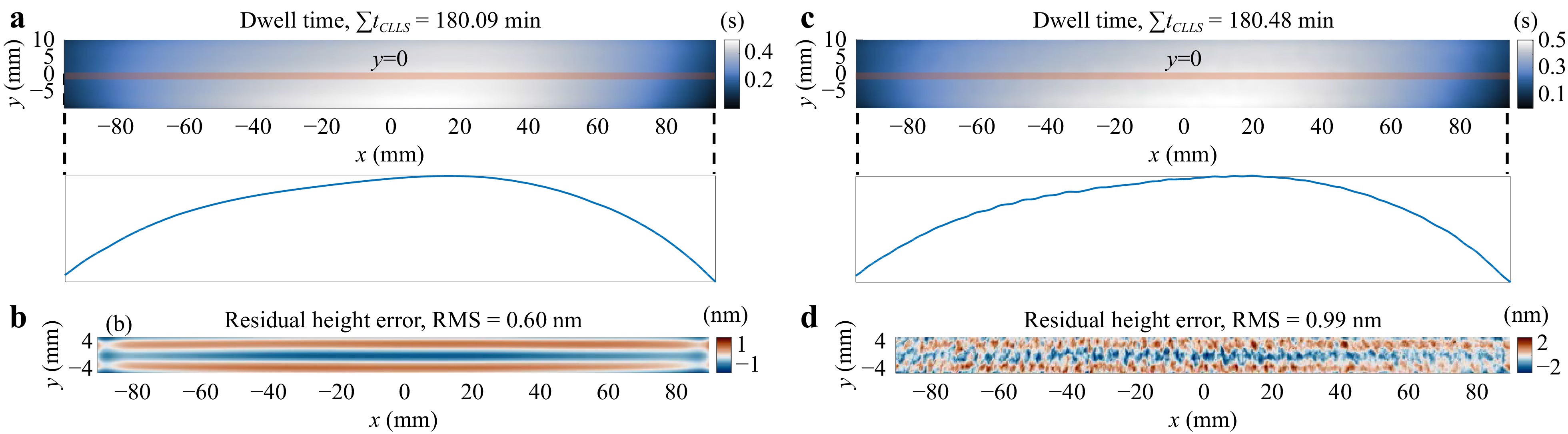
Fig. 13  Dwell time and residual height errors calculated using CLLS. a, b are the dwell time and residual height errors without the middle-frequency error (MFE) and high-frequency-error (HFE), respectively. c, d are the dwell time and residual height errors with MFE and HFE, respectively.

As shown in Fig. 13a, c, the dwell time maps obtained from both the cases with and without MFE and HFE resemble the shape of the nominal removal maps, with a slightly larger total dwell time than the ground truth. When comparing Fig. 13c with Fig. 12c, the dwell time profile with MFE and HFE present in CCLS is smoother than that in LSQR, thanks to the constrained optimization and coarse-to-fine scheme. However, introducing these improvements results in a higher computational burden of CCLS than LSQR.

On the other hand, the residual error maps, as shown in Fig. 13b, d, are slightly smaller than those obtained using LSQR. However, they are still less accurate than the other matrix-form dwell time optimization methods, indicating that the constraints fed into CLLS may still be sub-optimal. A possible improvement may be varying the difference constraints in $ {\bf{b}} $ by referencing the local slopes of $ {\bf{z}}_e $, however, incorporating this enhancement may increase the complexity of the CLLS method. Therefore, we leave this aspect for users to explore and experiment with in the future.

By closely examining MIM, RIFTA, and RISE, we have discovered an opportunity to further enhance matrix-form dwell time optimization by leveraging their advantageous strategies.

First, UDO borrows the arbitrary dwell points from MIM. The matrix-form update of dwell time in Eq. 34 is introduced to ensure that the dwell time can be iteratively refined to approach the convergence.

Moreover, UDO extends the simplifications of FIM proposed in RIFTA in Section 2.3.2 to simplify the MIM iterations in Eq. 34 by eliminating the $ {\bf{R}}^{{\rm{T}}}{\bf{R}}{\bf{t}}^{k} $ term. Building on this, as analogous to Eqs. 26 and 27, MIM can be modified by finding the optimal initial guess expressed in Eq. 36 as

where

As explained in Ref. 32, Eq. 45 implies that the computation of $ {\bf{t}} $ is equivalent to determining an optimized proportion of a pre-filtered surface error, denoted as $ {\bf{z}}_e $(i.e $ {\bf{R}}^{{\rm{T}}}{\bf{z}}_e $). Since the matrix $ {\bf{R}} $ is constructed with the TIF in each of its columns, this pre-filtering is a low-pass process, which inherently results in a smooth dwell time solution $ {\bf{t}} $, as elucidated in Section 3.1. However, as explained in Section 3.4.1, this pre-filtering process introduces unnecessary dwell time to each dwell point, which is eliminated in Algorithm 8 by an appropriate piston adjustment in each iteration.

Finally, in cases where only the CA data is available, the RISE concept can be employed to refine the dwell time solution iteratively through polynomial-based extrapolations. In the $ (k+1) $th ($ k\geq0 $) iteration, the RISE-based extrapolation is applied to the residual error $ {\bf{e}}_{CA}^{k+1}=\left({\bf{z}}_{e}-{\bf{R}}{\bf{t}}^{k}\right)_{CA} $ to obtain the target removal $ {\bf{z}}_{e|Poly}^{k+1} $, from which the incremental dwell time $ \Delta{\bf{t}}^{k+1} $ is calculated using Eqs. 45 and 46 as

which is then used to update the ($ k+1 $)th dwell time solution as

With the same smoothness and low-frequency correction assumptions illustrated in Fig. 2, the modifications from RIFTA, RISE, and MIM culminate in the proposal of UDO. UDO combines the benefits of RIFTA and RISE while incorporating the advantage of arbitrary dwell positions from matrix-form methods.

UDO is implemented in Algorithm 8, which is a “matrix-form” RISE except Line 13, where the zero-mean version of $ \Delta{\bf{z}}_{e|Poly}^{k+1} $, denoted as $ \Delta\bar{{\bf{z}}}_{e|Poly}^{k+1} $, is used for dwell time reduction. As analogues to Eq. 31 in RISE, this operation is necessary for UDO to eliminate the unnecessary increase of the total dwell time during iterations because of the pre-filtering process with $ {\bf{R}}^{{\rm{T}}} $.This is manifested by letting $ \Delta\bar{{\bf{z}}}_{e|Poly}^{k+1}=\Delta\bar{{\bf{z}}}_{e|Poly}^{k+1}-\mu $, where $\, \mu $ is the mean of $ \Delta\bar{{\bf{z}}}_{e|Poly}^{k+1} $. Eq. 47 can be rewritten as

where $ \boldsymbol{\mu}=\left[\mu,\mu,\ldots,\mu\right]^{{\rm{T}}} $. It can be observed in Eq. 49 that the distribution of $ \Delta{\bf{t}}^{k+1} $ is described by $ {\bf{R}}^{{\rm{T}}}\Delta\bar{{\bf{z}}}_{e|Poly}^{k+1} $, while $ {\bf{R}}^{{\rm{T}}}\boldsymbol{\mu} $ introduces constant dwell time to each entry in $ \Delta{\bf{t}}^{k+1} $ except the ones along the boundary, which is unnecessary and can be eliminated.

By doing so, in each iteration, $ {\bf{t}}^{k+1} $ has an equal possibility of positive and negative adjustment, and thus reduces the increase of the total dwell time. To keep the positivity of the final $ {\bf{t}} $, a piston adjustment is performed for $ {\bf{t}}^0 $ as shown in Line 3. If $ {\bf{t}} $ still contains negative entries after the iterative refinement, their magnitudes are always small and can be safely offset as $ {\bf{t}}={\bf{t}}-{\rm{min}}({\bf{t}})+t_{min} $³².

To solve Eq. 46, the same derivative-free optimization algorithms^{44, 45, 58} can be employed, since $ \gamma^{k+1} $ is the only unknown scalar to be optimized. A good initial guess for $ \gamma^{k+1} $ can be chose as the least-squares solution of $ \frac{1}{2}\left|{\bf{z}}_{e|Poly}^{k+1}-\gamma^{k+1}{\bf{R}}{\bf{R}}^{{\rm{T}}}\Delta\bar{{\bf{z}}}_{e|Poly}^{k+1}\right|^{2}_{2} $ as

We initially evaluate UDO on the nominal removal without MFE and HFE. The dwell time and the corresponding residual height error maps are demonstrated in Fig. 14a, b, respectively. Although the total dwell time is 25-min shorter than the ground truth, the residual error RMS is slightly higher than those of RIFTA, RISE, and MIM. The higher residual error can be primarily attributed to the pre-filtering process. Despite both UDO and RISE employing the same surface extrapolation method, there is a crucial distinction: UDO performs surface extrapolation on $ {\bf{R}}^{{\rm{T}}}{\bf{z}}_e $, while RISE does so on $ z_e $. The sparsity of matrix $ {\bf{R}} $ along the edges results in insufficient filtration, thus making UDO more susceptible to extrapolation errors.

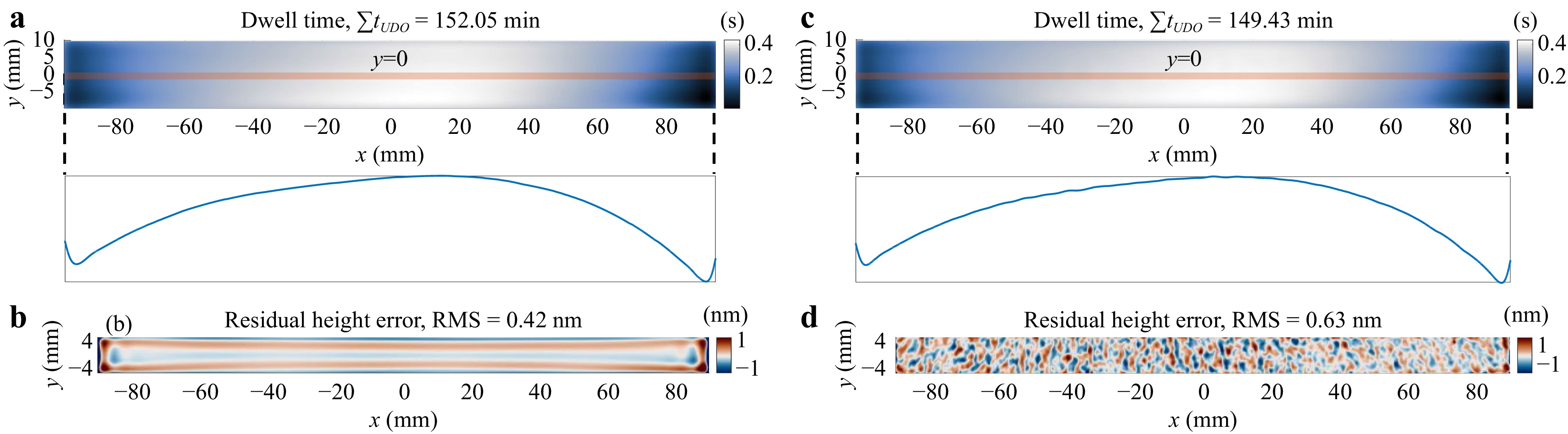
Fig. 14  Dwell time and residual height errors calculated using UDO. a, b are the dwell time and residual height errors without the middle-frequency error (MFE) and high-frequency-error (HFE), respectively. c, d are the dwell time and residual height errors with MFE and HFE, respectively. UDO handles MFE and HFE well and reduces the total dwell time.

Nevertheless, the extrapolation errors introduced by the pre-filtering strategy become negligible when dealing with surface errors containing MFE and HFE components. As illustrated in Fig. 14c, d, UDO consistently achieves a lower residual error RMS compared to RIFTA, RISE, and MIM in the presence of MFE and HFE. Additionally, in comparison with RISE, UDO not only attains a smoother dwell time profile but also maintains a similar total dwell time (only 5 mins longer), highlighting its effectiveness in handling MFE and HFE. Consequently, we recommend the use of UDO for matrix-form dwell time optimization. Integrating the advantages of RIFTA, RISE, and MIM in UDO results in a comprehensive approach that offers improved accuracy, efficiency, and flexibility in dwell time optimization for various CCOS processes.

In Sections 2 and 3, eight dwell time optimization methods have been reviewed. The optimized implementations and performance evaluations are demonstrated. Notably, it is worth recognizing that function-form methods are essentially special cases of matrix-form methods. All function-form methods can be solved within the matrix-form framework. The advantage of the function-form emerges mainly when the matrix $ {\bf{R}} $ is square. In this scenario, the function-form methods prove advantageous as the explicit construction of matrix $ {\bf{R}} $ becomes unnecessary, enabling the application of specialized function-form techniques.

To provide a comprehensive summary of the performance of the reviewed dwell time optimization methods, the results of applying these methods to the nominal removal map with MFE and HFE present are presented in Fig. 15, where their accuracy, total dwell time, dwell time smoothness, and computational efficiency are assessed. The statistics of the comparison of accuracy, feasibility, efficiency, and flexibility among the reviewed dwell time optimization methods are further detailed in Table 1. All the tests are performed on a workstation with an Intel Xeon Gold 5118 CPU (2 processors, 12 cores/processor, 2.30 GHz main frequency) and 256 GB RAM.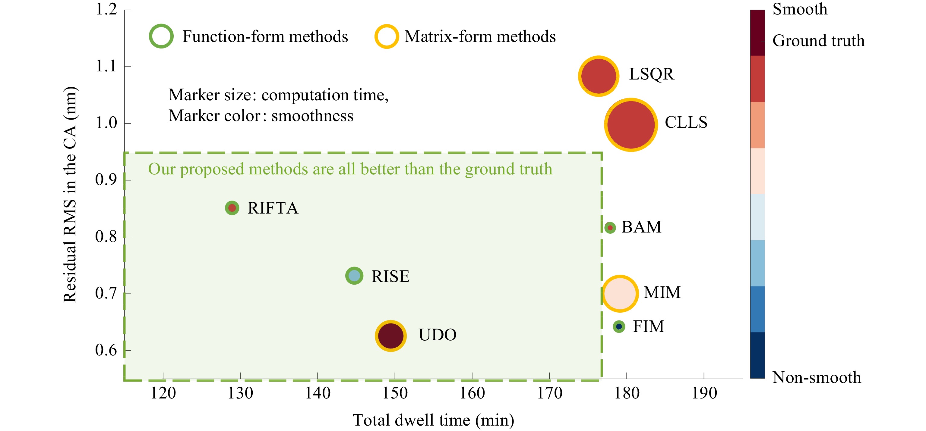

Fig. 15  Comparisons of residual error in the CA, total dwell time, dwell time smoothness, and computation time obtained from each of FIM, BAM, RIFTA, RISE, MIM, UDO, LSQR, and CLLS methods. The sizes of the circular markers indicate the computation time for each method and the colors denote the smoothness computed using Eq. (51). It is evident that RIFTA, RISE, and UDO attain the results better than the ground truth in terms of accuracy and processing efficiency.

While the accuracy and processing efficiency are referred to as the residual RMS in the CA and the total dwell time, respectively, the dwell time smoothness is quantitatively evaluated as the slope RMS magnitude of the profile of a dwell time map along the $ x $ direction at $ y=0 $, calculated as

where $ i=0,1,\ldots,524 $ is th $ i $th dwell point in the $ x $ direction. Finally, computational efficiency is measured by the computation time needed for each method and reflected by the sizes of the circular markers in Fig. 15.

Upon careful comparison, it becomes evident that the function-form methods, RIFTA and RISE, and the matrix-form method, UDO (as highlighted in Table 1), exhibit remarkable superiority over the ground truth in accuracy and processing efficiency. Notably, these methods have surpassed the ground truth benchmark, demonstrating outstanding performance in dwell time optimization.

In terms of accuracy, these methodologies have collectively achieved surface error RMS values at a sub-nanometer scale in the CA. This achievement signifies a notable enhancement over the ground truth value of 0.96 nm RMS. The convergence of these approaches towards sub-nanometer precision underscores their capability to yield exceptionally accurate dwell time solutions, elevating the standards of dwell time optimization. Furthermore, the processing efficiency of these methods is evidenced by their consistently shorter total dwell times compared to the ground truth.

Regarding computational efficiency, all the function-form methods, FIM, BAM, RIFTA, and RISE, are considerably faster than the matrix-form methods, namely MIM, UDO, LSQR, and CLLS. Among the function-form methods, FIM and BAM are the fastest methods. However, the smoothness of FIM’s result is not satisfactory. On the other hand, all the matrix-form methods demonstrate a similar level of smoothness in their results comparable to the ground truth. Nonetheless, these methods have a significantly heavier computational burden, particularly LSQR and CLLS. These methods require more computational resources and time to achieve accurate and smooth dwell time solutions.

Given these insights, we recommend consistently utilizing RIFTA and RISE for dwell time optimization when the dwell points are uniformly defined on a rectangular grid and refer to UDO when more flexible dwell positions are required. In the subsequent sections, we further encapsulate the strategies embedded within the reviewed dwell time optimization methodologies and other essential aspects. These strategies collectively achieve dwell time solutions characterized by accuracy, feasibility, efficiency, and adaptability.

Upon examination, it becomes apparent that all the optimized implementations of the reviewed methods, except CLLS, employ an iterative refinement procedure of dwell time. The CLLS method indeed includes an implicit refinement procedure in its active-set solver. Therefore, an iterative refinement procedure is crucial for minimizing residual errors in the CA, particularly in applications that prioritize ultra-precision, such as synchrotron X-ray mirrors and EUV lithography optics fabrication.

In cases where ample measurement data is available, the iterative updates are directly performed on the residual errors. However, when only the data in the CA is accessible, an iterative surface extrapolation technique (such as RISE or UDO)^{45, 32} can be performed to add additional data for the further refinement of the dwell time solutions.

There are two primary sources for the increase in the total dwell time. One is from the piston adjustment on the target removal map, $ z_e $, to ensure the non-negativity of the dwell time. This adjustment increases the overall dwell time by redistributing the removal amount. To solve this problem, the piston adjustment can also be iteratively performed with FIM or MIM⁴⁰. In each iteration, instead of using $ {\rm{min}}(z_{e}-r**t^{k}) $ to adjust the piston, a piston, $ p $, is added. When negative entries appear in $ t^k $, they are set to zero and rely on the next iteration for further refinement. The appropriate values for $ p $ can be set as $ \eta\cdot{\rm{RMS}}(z_e-r**t^k) $, where $ \eta>1 $.

The second factor arises from including unnecessary contributions of the dwell time outside the CA. In RIFTA, it has been proposed to perform the piston adjustment using only the data in the CA. As shown in Fig. 15, this adjustment is very effective and achieves a total dwell time even less than the ground truth.

It can be found that smoothness is enforced by incorporating smoothness assumptions in each dwell time optimization method. For example, BAM employs the Poisson distribution to model noise⁴², and RIFTA assumes that the initial dwell time solution is proportional to the target removal map. Also, the pre-filtering process proposed in the matrix-from methods helps smooth the target removal before performing dwell time optimization. As shown in Fig. 15, combining this pre-filtering process with the strategy proposed in RIFTA, UDO achieves the smoothest dwell time solution³².

Additionally, parameterizing the surface error with Zernike polynomials⁶¹ or B-spline surfaces⁶² before dwell time optimization helps improve the smoothness of dwell time solutions, owing to the inherently smooth and continuous properties of these parametric modeling methods. The smoothness of the dwell time solution can be controlled by the order of Zernike polynomials or the number of knots of the B-spline surface, which also determines the number of total dwell points and computational efficiency. In practice, an appropriate trade-off between the residual error and the number of dwell points should be made based on the complexity of the surface error, the computational efficiency, and the dynamics constraints of the machine tool.

As illustrated in Fig. 15, function-form methods are much more computationally efficient than matrix-form methods since FFT has been employed to accelerate the convolution operations. Even if the shape of a target removal map is irregular, as long as the dwell points are defined on a rectangular grid, we can still use FFT by excluding the invalid points from the final results (e.g., the nanfft function used in MATLAB).

However, when arbitrary dwell points are required, the matrix-form methods must be used, especially when we want to optimize dwell time for different machine tools simultaneously, the most computationally expensive LSQR or CLLS must be employed. While sparse-matrix structures should be used to save memory, the sub-matrix stitching method⁵² further reduces the computation time for large optics fabrication at the cost of decreasing the accuracy. Alternatively, the B-spline surface approximation method⁶² can be used to reduce the number of dwell points by the optimization of the knot positions during dwell time calculation.

A sophisticated CCOS system typically comprises multiple machine tools of varying types, shapes, and sizes, which allows for effective and efficient correction of surface errors with different spatial frequencies. Traditionally, the dwell time for each machine tool is sequentially calculated, optimizing it individually. However, this sequential approach fails to consider the overall contribution of multiple tools simultaneously^{11, 58}. As a result, the total dwell time is not well balanced among the employed tools, which can negatively impact processing efficiency.

In practice, although a CCOS process is usually scheduled using the TIFs with the sizes from big to small sequentially, the dwell time optimization can be performed non-sequentially for all the TIFs^{11, 31, 58} by taking advantage of the discretized, matrix-form formula as

where $ P $ is the number of TIFs and $ {\bf{R}}_i $ is the convolution matrix for the $ i $th TIF. This non-sequential system can be solved with either LSQR or CLLS. It considers all the TIFs simultaneously, which has been shown to reduce MFE and HFE errors while improving the smoothness of the dwell time solutions for each tool^{11, 31}. Moreover, the LSQR solution balances the total dwell time along different TIFs, thereby advancing the overall processing efficiency⁵⁸.

Furthermore, the matrix-form discretization can facilitate multi-objective optimization problems, where desired residual error criteria are set for height and slope^{5, 55, 60}. Instead of building separate $ {\bf{R}}_i $ matrices for different TIFs, $ {\bf{R}}_x $ and $ {\bf{R}}_y $ are utilized, representing the convolution matrices for the slopes of the TIF in the $ x $ and $ y $ directions, respectively. It has been discovered that an alternate objective optimization method associated with the LSQR solver can help achieve desired residual height and slope errors simultaneously more efficiently⁵.

The dwell time optimization methods reviewed in this study are further evaluated through an IBF experiment involving finishing an off-axis, elliptical-cylindrical mirror. As illustrated in Fig. 16a, the mirror is designed for hard X-ray focusing and has a CA size of 150 × 10 mm. The mirror’s off-axis ellipse geometry is depicted in Fig. 16b, with the specific parameters: object distance $ p=46.42 $ m, image distance $ q=0.33 $ m, and grazing angle $ \theta=2.2 $ mrad. This mirror has undergone pre-figuring using IBF, utilizing a TIF with a full-width half maximum (FWHM) of 4.7 mm. After pre-figuring, the residual target removal, as presented in Fig. 17a, is 6.48 nm RMS. Subsequently, the finishing process is carried out using the same IBF system but a smaller TIF, with an FWHM of 1.2 mm and a PRR of 3.2 nm/s, as shown in Fig. 17b. The desired residual error in the CA is specified as $ \leq0.5 $ nm RMS. To keep the comparison fair, the dwell points are distributed over the surface with the same sampling interval as the target removal map in Fig. 17a, which is 0.275 mm/pixel.

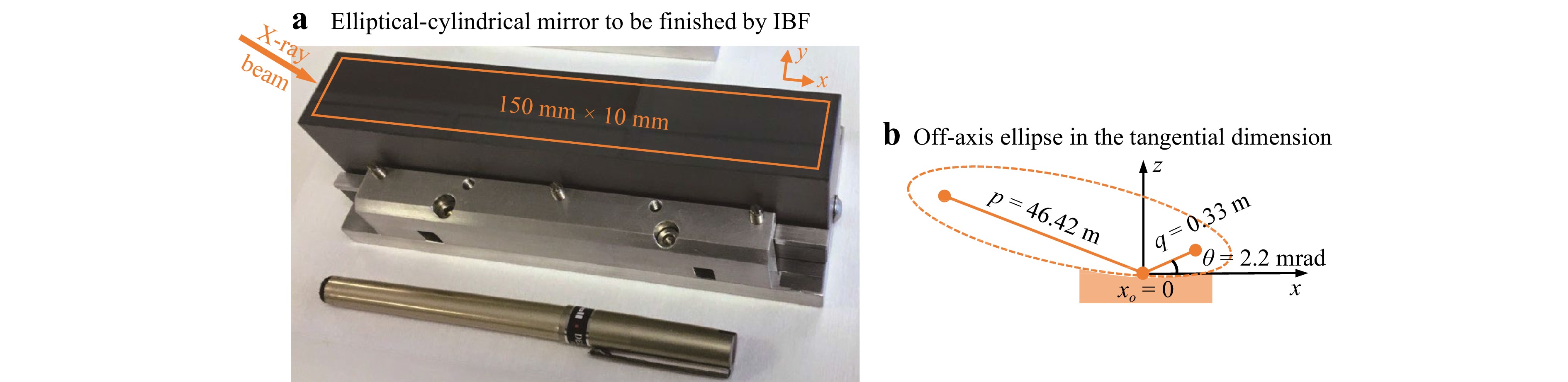
Fig. 16  a The elliptical-cylindrical mirror to be finished by IBF. b The geometry of the ellipse is the object distance $ p=46.42 $ m, image distance $ q = 0.33 $ m, and grazing angle $ \theta = 2.2 $ mrad.

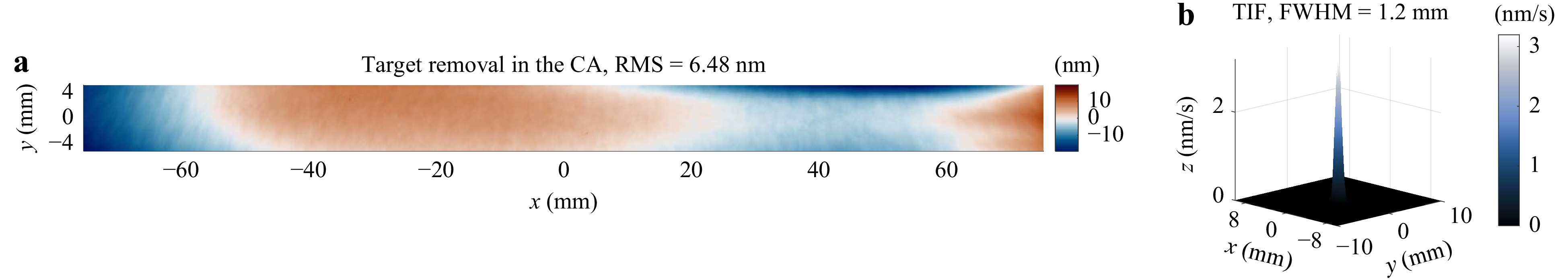
Fig. 17  a The target removal for the experiment is 6.58 nm RMS. b The IBF TIF used in the finishing has a FWHM = 1.2 mm and a PRR = 3.2 nm/s.

All eight dwell time optimization algorithms reviewed in this study are applied to the target removal and TIF given in Fig. 17. The dwell time solutions and estimated residuals obtained from these methods are compared. In the actual IBF experiment, only the dwell time solution achieving the best balance in accuracy, feasibility, efficiency, and flexibility is utilized to guide the finishing. This comprehensive evaluation aims to identify the most suitable dwell time optimization method that meets the specific requirements of the sub-nanometer-level IBF experiment, ensuring the results obtained from a real-world scenario coincide with the ones concluded from the simulation studied shown in Sections 2, 3, and 4.

The dwell time solutions optimized through FIM, BAM, RIFTA, RISE, MIM, UDO, LSQR, and CLLS are visualized in Fig. 18a–h, respectively. The corresponding estimated residual errors within the CA are shown in Fig. 18i–p respectively. The dwell time solution is analyzed based on the accuracy, feasibility, efficiency, and flexibility criteria below.

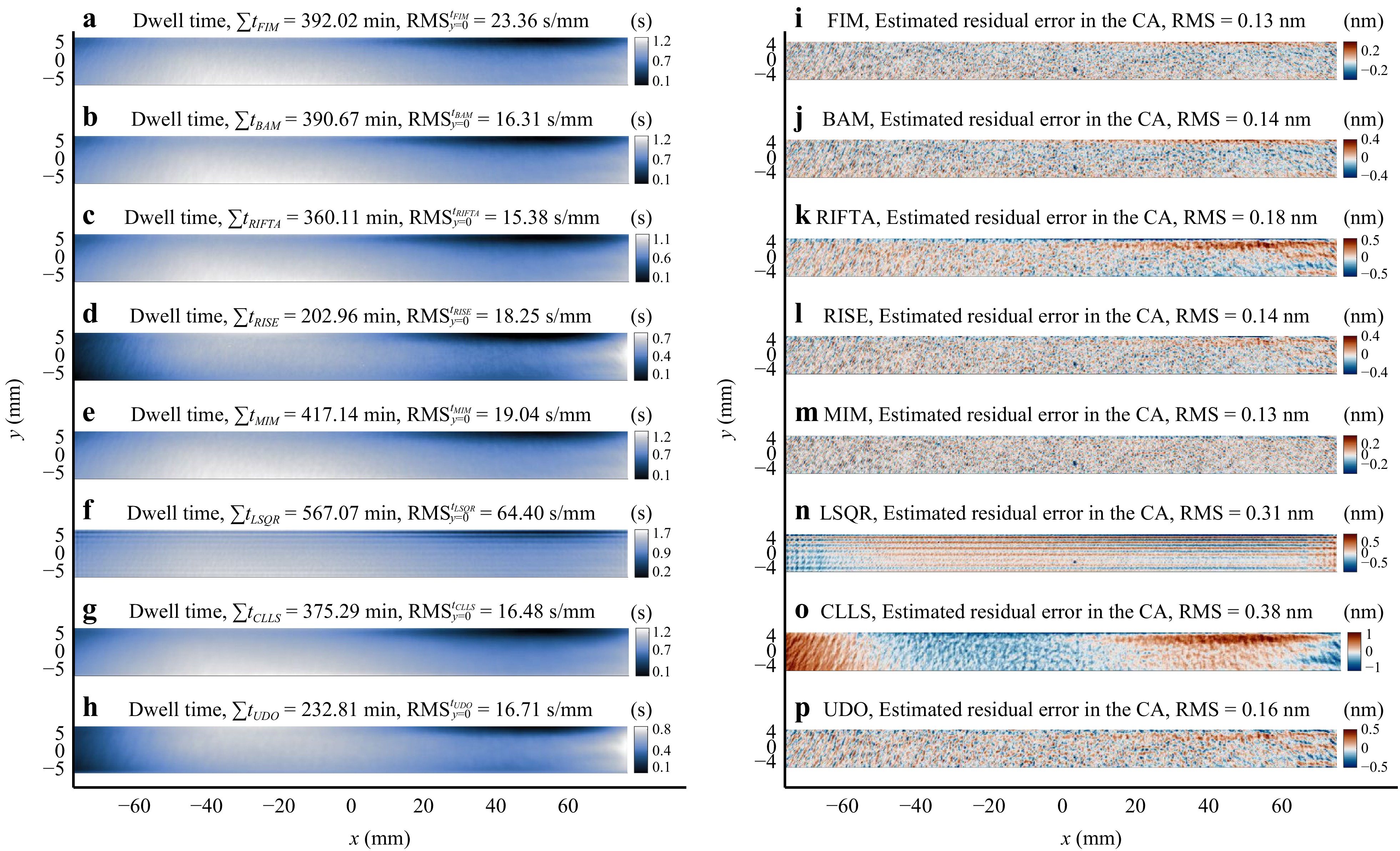
Fig. 18  Dwell time solutions a–h and the corresponding estimated residual errors in the CA i–p optimized using FIM, BAM, RIFTA, RISE, MIM, LSQR, CLLS, and UDO, respectively. It is evident that UDO achieves the best trade-off among algorithmic accuracy (0.16 nm RMS), feasibility ($ {\rm{RMS}}_{y=0}^{t_{UDO}}=16.71 $ s/mm), and processing efficiency ($ \sum t_{UDO}=232.81 $ min).

● Accuracy: In achieving sub-nanometer level finishing, the primary criterion for a reliable dwell time solution is its accuracy, as reflected by the residual error in the CA. From Fig. 18i–p, it is evident that all methods, except LSQR and CLLS, yield comparable levels of accuracy. The maximum RMS difference among the residual error maps is merely 0.05 nm, which can be considered negligible.

● Feasibility:

– Dynamics constraints: it is noteworthy that all the implementations presented in this study inherently account for dynamic constraints, ensuring the rationality of the resulting dwell time solutions.

– Smoothness: FIM has the largest slope RMS magnitude value of 23.36 s/mm, which indicates a insufficient smoothness and coincides with the conclusions in Table 1.

● Efficiency:

– Processing efficiency: From Fig. 18c, d, h, it can be observed that RIFTA, RISE, and UDO achieve the shortest total dwell time. Notably, the dwell time calculated by RISE and UDO is more than two hours shorter than that of RIFTA.

– Computational efficiency: the computation time of RISE and UDO, using the same computer illustrated in Section 4, is 7.1 s and 47.8 s, respectively, for a total number of 25,756 dwell points. Although the computation time of UDO is 40 s longer than RISE, we still keep it in our final dwell time solution list, as its smoothness (16.71 s/mm) is better than that of RISE (18.25 s/mm).

● Flexibility: as illustrated in Section 3, UDO is a matrix-form method featuring flexible dwell positions. Thus, the computation time of UDO can be reduced by using fewer dwell points. As shown in Fig. 19, if we use 0.5 mm as the dwell time interval, the number of dwell points is reduced to 8,289, while the total dwell time ($ \sum t_{UDO}=229.80 $ min, as shown in Fig. 19a), and the estimated residual in the CA (0.2 nm RMS, as shown in Fig. 19b) are very similar to those shown in Fig. 18h, p, respectively. The computation time for this dwell time solution is merely 16.8 s, comparable to that of RISE (2.4 times longer).

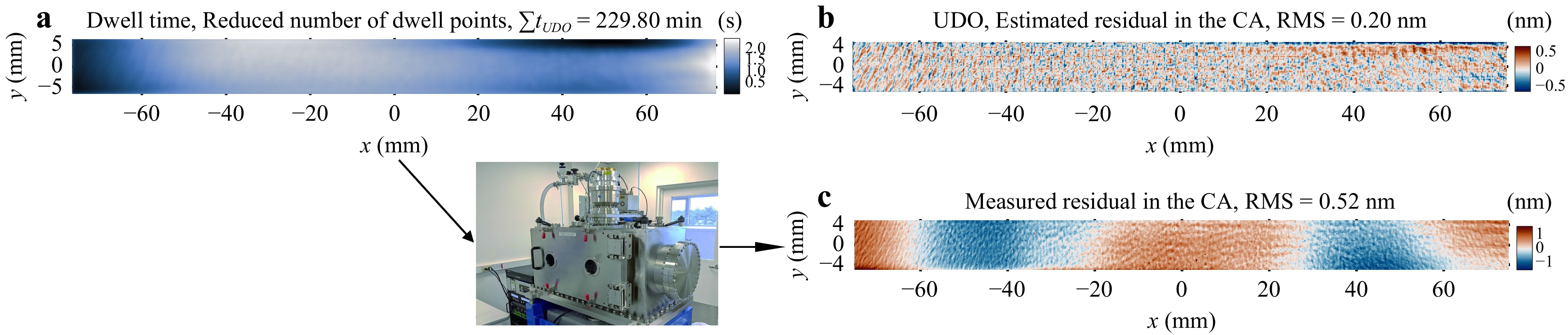
Fig. 19  a The dwell time optimized with UDO for the reduced number of dwell points (8,289) gives b an estimated residual error in CA of 0.20 nm RMS. This dwell time is sent to IBF for finishing the mirror. c The measured residual in the CA after the IBF process is 0.52 nm RMS.

Based on the above analysis, it is evident that the performance of the eight dwell time solutions applied in this experiment follows the same conclusions obtained from the simulation results shown in Fig. 15 and Table 1.

Finally, the dwell time solution presented in Fig. 19a is sent to IBF for finishing the mirror since it achieves a good balance among accuracy, feasibility, efficiency, and flexibility. After the IBF process, the actual measured residual error in the CA is 0.52 nm RMS, which meets the specification, and thus the finishing is completed. It is worth mentioning that there is a discrepancy between the estimated and actual residual errors in the CA, as shown in Fig. 19b, c, respectively. This discrepancy has mainly resulted from the uncertainties during the IBF process, such as thermal effect⁸⁵, motion control⁸⁶, positioning accuracy⁸⁷, TIF stability^{88, 89}, etc., each of which is an active research topic in modern, deterministic CCOS systems. This study only restricts its discussion to the algorithmic performance of dwell time optimization, aiming to minimize the optimization errors' contribution to the actual CCOS process.

We have conducted a thorough review and comparison of various dwell time optimization methods for CCOS, encompassing theoretical analysis on the internal mechanisms, uncovering their relationships, and exploring implementation strategies. The performance of these methods is evaluated across accuracy, feasibility, efficiency, and flexibility, with results further validated through simulation and experimentation. It is now worth reiterating the connections among the reviewed methods illustrated in Fig. 2 and providing suggestions on selecting a proper dwell time optimization method for different CCOS processes.

FIM^{10, 37-41} pioneers dwell time optimization for CCOS. All the other methods can be derived from FIM and they share the same convergence criteria. The additive iterative process of the dwell time within FIM converges when satisfying Eqs. 10 and 11. However, in the presence of MFE and HFE (or noise), the smoothness of the dwell time is compromised. Addressing this challenge, BAM^{28, 42} models the noise as a Poison distribution, treating deconvolultion as a Bayesian process. BAM, an iterative algorithm like FIM, differentiates in its approach by employing multiplicative iterations, resulting in a smoother dwell time solution. Furthermore, we demonstrate that in the absence of noise, FIM converges to FTM^{20, 38, 43}, where dwell time is solved through an inverse filtering process. However, due to unavoidable noise in actual measurements, a threshold is introduced in FTM to filter out the high-frequency components during inverse filtering. Selecting an optimal threshold value is crucial for FTM, as an inappropriate choice may amplify noise, leading to an unstable dwell time solution. To address this issue, RIFTA⁴⁴ introduces an optimization algorithm to find the optimal threshold value. Additionally, employing an iterative refinement strategy, RIFTA refines the dwell time to reduce the total dwell time and estimated residual error simultaneously. Afterwards, RISE⁴⁵ introduces an iterative surface extrapolation scheme to handle the edge effects when only the CA data is available during the measurement process.

The aforementioned methods assume that the dwell points are defined on the same regular grid as the surface. However, when dealing with arbitrary dwell points or irregular surface shapes, matrix-form methods become necessary. In this context, the matrix-based discretization in Eq. 2 is employed. The simplest among these matrix-form methods is MIM⁴⁹, which is a direct extension of FIM. The convergence criteria of MIM in matrix-form are provided in Eqs. 33 and 35. An additional advantage of MIM is its pre-filtering process in Eq. 34, where multiplication with $ {\bf{R}}^{{\rm{T}}} $ acts as a low-pass filter, resulting in a smoother dwell time solution. Alternatively, the linear system in Eq. 2 can be directly solved. However, due to the near singularity of the matrix $ {\bf{R}} $, solvers often involve Tikhonov regularization^{11, 16, 17, 29, 30, 31, 50-58} or CLLS^{30, 59, 60} methods to ensure a reasonable dwell time solution. Tikhonov regularization often takes the form of a TSVD problem, but due to its computational burden, a more efficient LSQR solver⁸² has been introduced. On the other hand, CLLS addresses the linear system by incorporating necessary constraints, with the added benefit of considering the actual dynamic constraints of a CCOS machine. However, both LSQR and CLLS suffer from low computational efficiency and may lead to unsmooth dwell time solutions. To overcome these challenges and achieve both computational efficiency and smooth dwell time solutions in matrix-form, UDO³² combines the strengths of MIM with the strategies proposed in RIFTA and RISE. Instead of directly solving Eq. 2, UDO calculates dwell time by determining the optimal proportion of the pre-filtered surface error, i.e., $ {\bf{R}}^{{\rm{T}}}{\bf{z}}_e $. Finally, it integrates dwell time reduction and surface extension schemes from RIFTA and RISE, resulting in a smoother dwell time solution with reduced total dwell time.

Utilizing the mechanistic analysis presented in Fig. 2 and detailed discussions in Sections 2 and 3, along with insights from simulation and experimental results illustrated in Fig. 15 and Table 1, we offer guidance for selecting an appropriate dwell time optimization solver in practical CCOS processes. As illustrated in Fig. 20, two aspects need to be considered in a practical CCOS process: the problem scale and the distribution of dwell points.

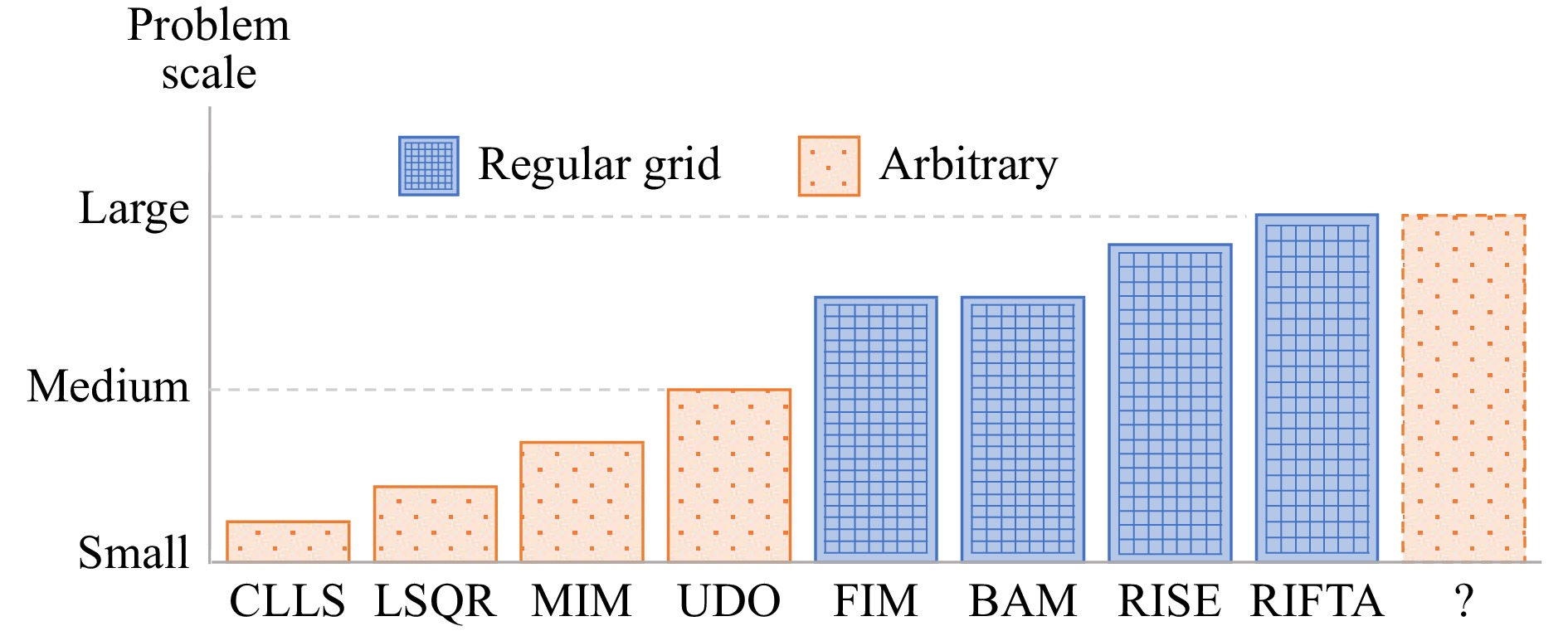
Fig. 20  Guidance of the choice of a dwell time solver by considering both the problem scale and the distribution of dwell points. Further exploration is needed for a dwell time solver capable of effectively handling large-scale problems and accommodating arbitrary dwell positions.

For smaller problem scales, all methods are viable, delivering comparable accuracy (see Fig. 18). However, as the problem scale increases, conventional matrix-form methods (CLLS, LSQR, and MIM) become impractical due to their substantial computational burden. When dwell points are distributed on a regular grid, function-form methods (FIM, BAM, RIFTA, and RISE) are applicable. For cases requiring arbitrary dwell positions and addressing descent problem scales, UDO stands out as a suitable choice. Nevertheless, there remains a gap in dwell time algorithms capable of handling both large problem scales and arbitrary dwell point distributions. Concerning further enhanced smoothness and shorter total dwell time, we recommend employing RIFTA, RISE, and UDO for reasonably sized problems. For matrix-form methods seeking further smoothness, post-processing steps such as Zernike mapping⁶¹ or B-spline fitting⁶² can be applied to the calculated dwell time.

This paper comprehensively reviews eight well-known dwell time optimization methods, classified into function-form and matrix-form methods. The key contributions of this study are summarized as follows.

First, the study provides a detailed exposition of the principles underlying each of the eight dwell time optimization methods. This involves a thorough mechanistic analysis and explanation of the strategies embedded in each method. Notably, the study unveils, for the first time in the literature, the close interconnections between these methods, shedding new light on their shared principles.

Second, the study proposes optimized implementation for each method based on our best knowledge, enhancing their practical applicability.

Third, the performance of these optimized implementations is comprehensively assessed using nominal removal maps generated from a ground truth dwell time. The evaluation is based on four critical criteria for assessing dwell time solutions: accuracy, feasibility, efficiency, and flexibility, providing readers with a deeper understanding of the relationship between the principle and practical performance of each method.

From the simulation results, it is concluded that the function-form methods, namely the robust iterative Fourier transform-based dwell time optimization algorithm (RIFTA) and robust iterative surface extension (RISE), in conjunction with the matrix-form method, universal dwell time optimization (UDO), achieved the most favorable balance across the four criteria. Therefore, we recommend users considering these three methods for future applications in computer-controlled optical surfacing, as they collectively represent optimal solutions with superior performance in the aspects of accuracy, feasibility, efficiency, and flexibility.

This work was supported by the Accelerator and Detector Research Program, part of the Scientific User Facility Division of the Basic Energy Science Office of the U.S. Department of Energy (DOE), under the Field Work Proposal No. FWP-PS032. This research was performed at the Optical Metrology Laboratory at the National Synchrotron Light Source II, a U.S. DOE Office of Science User Facility operated by Brookhaven National Laboratory (BNL) under Contract No. DE-SC0012704. This work was performed under the BNL LDRD 17-016 “Diffraction limited and wavefront preserving reflective optics development.” This work was also supported by the Natural Science Foundation of Fujian Province, China, under grant number 2022J011245.