Accuracy characterization of Shack–Hartmann sensor with residual error removal in spherical wavefront calibration

As an optical wavefront measurement system¹, the Shack–Hartmann wavefront sensor (SHWFS) has been widely used in fields such as adaptive optics^2-4, laser beam characterization⁵, ophthalmology^6,7, and quality control in optics fabrication including high-numerical-aperture microscope objectives⁸. Wavefront measurement using an SHWFS is based on the measurement of the local slopes of a distorted wavefront relative to a reference wavefront. The SHWFS must be calibrated by the reference wavefront before operation^9-11. The error in the reference wavefront directly affects the wavefront measurement results and cannot be eliminated¹². In 2005, Pfund et al.¹³ proposed for the first time use of spherical wavefronts generated by a single-mode fiber as the reference wavefront to calibrate an SHWFS; the calibrated SHWFS achieved an accuracy within λ/100 (λ = 657 nm) peak-to-valley (PV) across a diameter of 6 mm. Mercere et al.¹⁴ used a commercial SHWFS calibrated by a spherical wavefront to measure the wavefront aberration of an extreme ultra-violet lithography system; the root mean square (RMS) of the measurement repeatability was greater than λ/120 (λ = 13.4 nm).

An SHWFS comprises an array of microlenses and a photodetector placed on the focal plane of the array¹⁵. Its wavefront measurement accuracy is affected by the reference wavefront used for calibration, and errors of the sensor itself¹⁶, including manufacturing errors of the microlens array (MLA), response errors of the photodetector, and errors induced by sensor assembly¹⁷. Jiang et al.¹⁸ analyzed the systematic errors of an SHWFS and proposed that random errors mainly originated from the photodetector, including the readout noise, background electrical level, and photon noise. Jiang et al.¹⁹ analyzed the theoretical limit of wavefront measurements for an SHWFS and indicated that the measurement accuracy of the SHWFS was related to the photodetector noise and deviation of the focal spots from the MLA.

An spherical wavefront generated from a single-mode fiber can be used as the reference wavefront to calibrate an SHWFS, which can measure disturbed wavefronts with an accuracy of λ/100 PV. However, such a spherical wavefront has aberrations that cannot be eliminated by calibration; residual errors of the sensor inevitably produce uncertainty in wavefront measurement, which is unacceptable for highly accurate measurements of wavefronts in extreme manufacturing²⁰ including lithography lenses²¹ and astronomical telescope systems²². New methods for accurately calibrating an SHWFS must be developed.

In this study, based on the principle of spherical wavefront calibration of an SHWFS, a micrometer-scale pinhole with a diameter of 1 µm was used to generate spherical wavefronts with extremely small wavefront errors, with residual aberrations of 1.0 × 10⁻⁴ λ RMS, providing a high-accuracy reference wavefront. In the first step of SHWFS calibration, we used a modified method to solve for three important parameters (f, the focal length of the MLA, p, the sub-aperture size of the MLA, and s, the pixel size of the photodetector) to scale the measured results of the SHWFS. With only three iterations in the calculation, these parameters can be determined as exact values, with convergence to an acceptable accuracy. For a simple SHWFS with an MLA of 128 × 128 sub-apertures in a square configuration and a focal length of 2.8 mm, a measurement accuracy of 5.0 × 10⁻³ λ RMS was achieved across the full pupil diameter of 13.8 mm with the proposed spherical wavefront calibration. The accuracy is dependent on the residual errors induced in manufacturing and assembly of the SHWFS. After correcting these residual errors in the measured wavefront results, the accuracy of the SHWFS increased to 1.0 × 10⁻³ λ RMS, with measured wavefronts in the range of λ/4. Mid-term stability of wavefront measurement was confirmed, with residual deviations of 8.04 × 10⁻⁵ λ PV and 7.94 × 10⁻⁵ λ RMS. This study demonstrates that the modified calibration method of a high-accuracy spherical wavefront generated from a micrometer-scale pinhole can effectively improve the accuracy of an SHWFS; further accuracy improvement was verified with correction of residual errors, making the method suitable for challenging wavefront measurements such as in lithography lenses, astronomical telescope systems, and adaptive optics.

Fig. 1 shows the experimental setup for calibrating an SHWFS with a spherical wavefront. A semiconductor laser with a center wavelength of 0.635 μm was used as the light source and coupled to a polarization-preserving single-mode fiber (SMF) through an FC-PC connector. The light beam output from the SMF was focused using relay optics consisting of two doublets with focal lengths of 200 mm in a 4-f arrangement. A pinhole with a diameter of 1 μm was located on the focal plane of the relay optics to generate spherical wavefronts. Using the diffraction of the pinhole, highly accurate spherical wavefronts were produced, as shown in the upper-right corner of Fig. 1.

Fig. 1  Experimental setup for spherical wavefront calibration. SMF: single-mode fiber; Relay optics: two doublets with a focal length of 200 mm in a 4-f arrangement; SHWFS: Shack–Hartmann wavefront sensor.

To calibrate the SHWFS, the quality of the spherical wavefront as a reference source must be ensured. Traditionally, spherical wavefronts diffracted from an SMF are influenced by aberrations across the aperture of the sensor. For example, a normal SMF with a core diameter of 4 μm provides a spherical wavefront with estimated aberrations of λ/100 across the sensor with an aperture of 5 mm and a radius greater than 2 m. In our experiments, additional relay optics and pinholes were used to minimize the residual aberrations of the spherical wavefronts.

Theoretically, a smaller pinhole diameter results in a smaller spherical wavefront, influenced by aberrations across the pinhole aperture. When the aperture of the spherical wavefront is 0.2, the diameter of the pinhole must be less than 1.5 μm to produce an spherical wavefront error less than 10⁻⁵ λ (PV value)²³. Considering the influence of pinhole thickness, system alignment error, and beam propagation loss²⁴, the focused ion beam (FIB) etching mode was used to produce a 1-μm pinhole with a diameter accuracy of 10%. It was prepared on a 200-μm quartz plate with a chromium thickness of 200 μm.

According to the Fraunhofer diffraction integral¹³, the aberration error ΔΦ of an spherical wavefront diffracted from a pinhole can be described using Eq. 1.

where D is the aperture of the SHWFS; d₀ is the pinhole diameter; R₀ is the radius of curvature of the spherical wavefront, and ΔΦ₀ is the initial wavefront error of the pinhole. For relay optics in a 4-f arrangement with two doublets with a focal length of 200 mm, an estimated initial wavefront error ΔΦ₀= 0.01 λ is identifiable in the diffraction limit. The residual error ΔΦ of the spherical wavefront across the full aperture of the SHWFS with D = 13.8 mm was less than 1.0 × 10⁻⁴ λ RMS, as the distance R₀ was not less than 1.0 m in this setup. Thus, the quality of the spherical wavefront was assured; it was used as a highly accurate reference wavefront for SHWFS calibration.

When the highly accurate spherical wavefront surface is divided into several beamlets by the sub-apertures of the MLA in the SHWFS, spots focused on the photodetector are equally spaced in the row and column directions, as shown in Fig. 2. The distance Q of the spots on the photodetector can be expressed by N in pixels as

Fig. 2  Geometrical SHWFS principle: Side view, transverse centroid (x and y components) positions formed by the MLA on the photodetector. Top view, spot pattern formed by spherical wavefront on SHWFS photodetector; the pixels are depicted as gray squares.

To realize wavefront measurements with an SHWFS, the spot distance Q was used to calculate the spot slopes with the focal length of the MLA. Thus, the first step in accurate measurement of wavefronts is to determine the exact parameters of the SHWFS, which include f = focal length of the MLA, p=sub-aperture size of the MLA, s=pixel size of the photodetector.

Thus, with the known value R in a highly accurate spherical wavefront, by measuring the curvatures of the spherical wavefronts for several different radii, the values of f, p, and S can be determined using a least-squares algorithm, as described previously^13,16. As shown in Fig. 2, the radius of curvature R of the spherical wavefront is equal to the distance L between the origin (pinhole location in Fig. 1) of the spherical wavefront and the plane of the MLA of the SHWFS in the ideal case. In practice, it is difficult to confirm the exact position of the MLA with the required accuracy owing to the manufacturing process of the SHWFS. However, the position of the pinhole producing the spherical wavefront can be accurately measured. Thus, it is possible to precisely measure the distance between the two positions of the spherical wavefront.

An approximation L₀ that could be initially measured was used to determine the origin of the spherical wavefront. A series of distances L_i (i = 1, 2, 3, ..., K) on the housing of the pinhole that provided the spherical wavefront and the spot distance N_i (i = 1, 2, 3, ..., K) on the photodetector were recorded. For each pinhole position, we obtain

Thus, the parameters of the SHWFS can be solved using the least-squares algorithm.

For identification of all parameters, at least four equations are required to solve for f, P, S, and L₀, which means that at least four different locations L_i of the spherical wavefront are required to measure the spot distance N_i. Considering the nonlinearity of the parameters in Eq. 4 and the measurement noise, more than 10 pinhole locations were used in the experiment.

In Eq. 4, the relationship between N_i and the other parameters is nonlinear, which may yield unsuitable results through least-squares fitting. In fact, there is a tightly coupled relationship between the parameters P and S. Let

Eq. 4 becomes

Eq. 5 is decomposed into two steps for calculations:

In the first step of the SHWFS parameter calculation, an initial value T can be set with nominal values P and S in the design; the exact values of f and L₀ are solved in Eq. 6-1. Second, the value of T is determined using Eq. 6-2, as approximations of parameters f and L₀ are assumed. Thus, with only three calculation iterations, the best values for the parameters p, f, and L₀ can converge to acceptable accuracy. The sub-aperture size p of the MLA and the pixel size s are not independent, but have a tightly coupled relation in Eq. 3. Thus, it was impossible to calculate these values. As the errors in the photodetector were almost negligible, the pixel size s was maintained at the nominal value in its design; the exact value for the parameter p was calculated.

As shown in Fig. 1, all components in the experimental setup were installed on a linear guiderail; the SHWFS to be calibrated was fixed at the end of the guiderail. The other components including the laser, the SMF, the relay optics, and the pinhole were installed on a stage with a positioning accuracy of 1 μm that could move with a resolution of 200 nm along the guiderail to produce spherical wavefronts with different radii. A grating ruler with a reading head was mounted on the side of the guide to accurately record the pinhole position.

Thus, calibration of an SHWFS with spherical wavefronts consists of the following steps.

(1) Produce spherical wavefronts with different curvatures by moving the stage far from the SHWFS with radii of curvature greater than 1 m.

(2) Mathematically calculate f and P by measuring the spot array.

(3) Determine the residual errors of the SHWFS due to sensor manufacturing and assembly.

(4) Correct residual errors in the SHWFS to improve its accuracy.

The wavefront measurement accuracy of an SHWFS is decreased by manufacturing and assembly defects such as imperfections in the MLA and photodetector, and also by environmental disturbances and discrete sampling errors of the MLA. Prior to calibration, errors such as environmental disturbances must be strictly controlled as much as possible.

The experimental setup shown in Fig. 1 was installed on an optical platform with air flotation stabilization devices to effectively eliminate the effect of vibration. A shielding curtain was installed to prevent airflow disturbance. The temperature and humidity of the SHWFS must be kept within 22 ± 1°C and 50% ± 5%, respectively. Variation of temperature should be within 2 °C in one day. To prevent background light from entering the SHWFS, a retractable hollow cylinder was set between the SHWFS and pinhole, preventing spot detection errors. Prior to the experiments, the SHWFS was warmed up for more than 30 min.

The SHWFS used in this study was selected for its high resolution, with an MLA of 128 × 128 sub-apertures. Due to the limited spatial sampling of the wavefront with an MLA in an SHWFS, discrete sampling errors of wavefronts were inevitable; they were less than 0.1‰. For wavefront measurements with aberrations of 100 nm, the sampling error was less than 0.01 nm, which did not affect the accuracy of the wavefront measurement.

The SHWFS design parameters used in this study are presented in Table 1.

According to the calibration procedure in Section 2.3, the initial location value L₀ for the pinhole was set to 1060 mm, as shown in Fig. 1; 13 highly accurate spherical wavefronts were produced with gradually increasing curvature radii at 20-mm intervals. Spot images were obtained from the SHWFS. For each measurement of the spherical wavefronts, 100 frames of spot images were averaged to eliminate the impact of environmental disturbances. The p-values of the spot positions on the SHWFS were calculated in the x and y directions.

The experimental process was repeated five times; five groups of data for spot positions P and relative distances L₀ were obtained. According to Eq. 6-1, five groups of focal lengths f (in the x- and y-directions) of the MLA and the exact location values L₀ for the pinhole were calculated. Using the exact values of f and L₀, the values of T=$ P/S $ (in the x- and y-directions) were calculated using Eq. 6-2. The focal length f, position of the pinhole L₀ for the wavefront, and T are shown in Table 2.

Using highly accurate spherical wavefronts to calibrate the SHWFS across the full aperture, the exact parameters of the sensor were determined using the proposed calculation method. However, residual errors in the SHWFS were still present due to imperfections in the MLA and photodetector and sensor assembly errors; they are analyzed in this section.

To calibrate an SHWFS, the quality of the spherical wavefront must be ensured. As shown in Fig. 1, the spherical wavefront was diffracted from the pinhole; spherical wavefronts with different curvature radii R were generated by changing the pinhole position far from the SHWFS. Thus, even a small positioning error in the pinhole can affect the quality of the spherical wavefront. At a distance R for the curvature radius of the spherical wavefront, if there is an uncertainty of amplitude δZ for the axial positioning of the pinhole, an additional defocus aberration Δφ is induced in the spherical wavefront as

where r is the aperture radius of the SHWFS. For a high-accuracy stage (to be mounted with the pinhole) with a positioning accuracy δZ = 1 μm, the RMS value of residual defocus aberrations across the size of the SHWFS with r = 6.9 mm was less than Δφ = 10⁻⁵ λ for R ≥ 1.0 m and λ = 0.635 µm. Compared to the measurement accuracy of the SHWFS, the additional defocus aberration for the spherical wavefront resulting from the pinhole position error was negligible.

The presence of photon noise and readout noise can lead to centroiding errors in an SHWFS. Locally, additional errors arise from non-uniform responses of the pixels of the photodetector, resulting in random jitter of the measured spot positions. The errors in the photodetector response must be analyzed.

Prior to assembling the SHWFS, the photodetector response was measured using a uniform beam with a plane wavefront generated by an integrating sphere, as shown in Fig. 3a. There was a higher response in the areas near the center of the photodetector than in the surrounding areas; some bright lines crossed the full aperture of the detector, indicating inconsistent responses of these pixels. For a photodetector with an average gray value of 3200 ADU, the gray values in Fig. 3a were fitted to calibrate the response efficiency of all pixels; the residual variance of the photodetector decreased from 41 ADU to 2.4 ADU. The photodetector response with calibration is shown in Fig. 3b; the differences in the pixel responses across the aperture of the photodetector were almost eliminated.

Fig. 3  a Original response of photodetector used in this SHWFS; b Uniform response of the photodetector with calibration.

After determining the incident spot positions on the photodetector, the wavefront was reconstructed using the first partial derivatives calculated from the centroid positions of the measured and reference spots. The centroid offset was detected using an offset estimation algorithm in the Fourier domain (FDO)⁶. The calculation was converted from the spatial domain to the Fourier domain through a fast Fourier transform (FFT). The offset was calculated by selecting the part with a high signal-to-noise ratio according to the characteristics of the energy distribution of the signal and noise in the Fourier domain.

The FDO algorithm is unbiased and more efficient in noise suppression but is still affected by noise, including photon noise and readout noise²⁵. With photodetector calibration, the non-uniform response error of the pixels can be directly removed, which helps reduce photon noise. To improve the accuracy of the centroid, the intensity of the spot must be adjusted appropriately, typically set at 90–95% of the peak photodetector response. In addition, an estimated value of the optimum threshold for the centroid spots was determined in our experiments²⁶, which was favorable for suppressing photon noise.

Even with precision manufacturing technology, there are inevitably residual errors in the MLA, such as deviations from the nominal size of the sub-apertures, nonorthogonal errors in which the row and column directions are not exactly perpendicular, and defects in the shape and surface of some microlenses. Benefiting from high-precision fabrication, the MLA chosen for this study had an acceptable consistency in the size, shape, and surface of the microlenses. Most residual errors occur in rotation of the orthogonal x and y axes. This error causes the positions of the focal spots corresponding to the reference wavefront to deviate from the equidistant grid defined by the center of an ideal MLA, which can directly lead to errors in any wavefront measurement.

With the MLA used in this SHWFS, the positions of the focal spots deviated from the lines of the ideal matrix; periodic strips appeared in the x- and y-directions, as shown in Fig. 4. The high-precision mask for the MLA defines the ideal position of each sublens; the distance at which each sublens deviates from its ideal position is the error in that sublens. As shown in Fig. 4a, the sublens errors in the x-direction are stripe-shaped and have a periodic arrangement, indicating that all sublenses in this direction have a relatively consistent offset. For the sublenses in the y direction, there was a larger error near the edges, and the error shift directions on both sides were opposite, as shown in Fig. 4b. The error of the pitch of a single sub-lens was within ±0.05 μm; the accumulated error of all sub-lenses was less than 1 μm.

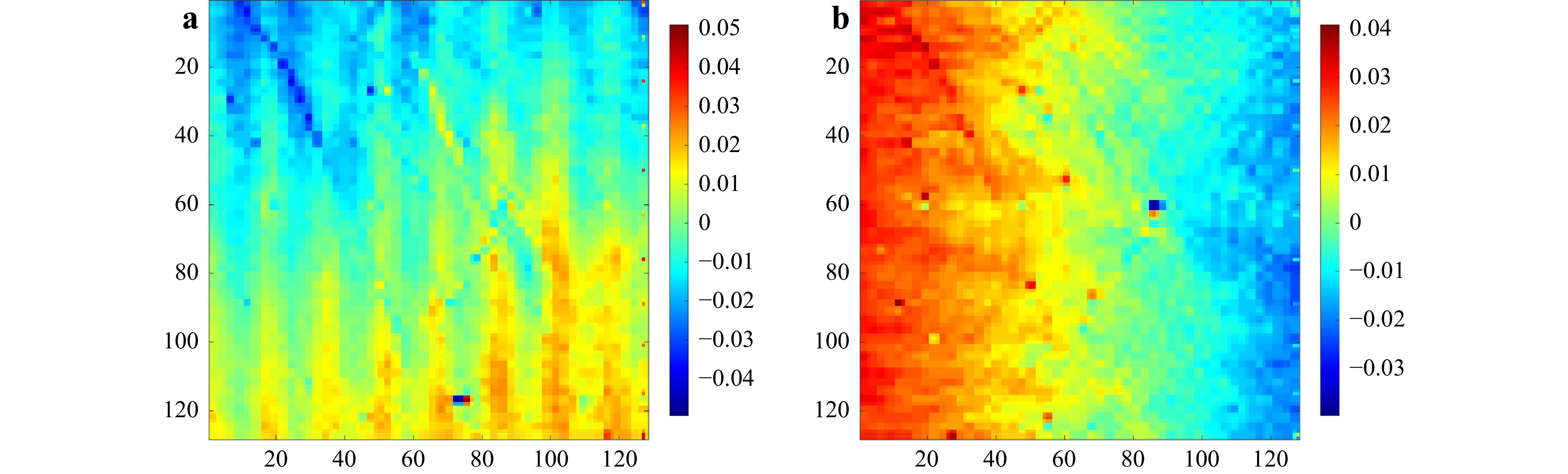
Fig. 4  Deviation from equal spacing caused by fabrication error in MLA: Periodic stripes were formed in the x-direction a and y-direction b.

To eliminate this error, a uniform wavefront generated from an integrating sphere was used in the first step to measure the exact positions of the focal spots. Individual deviations from the ideal focal spot were strictly calculated using the FDO centroiding algorithm^6,7; the measured positions of the MLA were recorded as the referenced matrix. Thus, the errors in the MLA can be eliminated for measurement of any wavefront.

In the process of integrating the SHWFS, a photodetector was placed on the focal plane of the MLA. Residual errors resulted from the limited accuracy of the assembly. These errors included the tilt between the MLA surface and the photodetector surface, and the coordinate axis rotation between the MLA and the photodetector.

The Zernike polynomials in Cartesian coordinates are presented in Table 3; the spherical wavefront used for the calibration can be expressed as

To verify the estimation of tilt errors, we measured the tilt angle between the MLA and the photodetector surfaces. The tilt angle can be expressed as slopes (a, b) in the x- and y-directions. A mathematical derivation yields the tilt error as

According to the data in Section 3.2, the tilt error $ {\Delta }W(\mathrm{x},\mathrm{y}) $ can be measured through the five groups of known spherical wavefronts W (x, y). The tilt angle between the MLA and the photodetector was calculated, as shown in Table 4.

By determining the tilt angle between the MLA surface and the photodetector surface, the focal length $ f $ of the MLA can be influenced by

The variance of the tilt angle between the MLA surface and the photodetector surface was large, but the averaged value was small. Thus, it can be considered that the residual tilt angle between the MLA and the photodetector was very small, not sufficient to cause a wavefront measurement error in the SHWFS; thus, this residual error can be ignored.

When a spherical wavefront was used to calibrate the SHWFS, a residual aberration of astigmatism with an angle of 45° was observed in the measured result once there was an additional rotation angle $ \theta $ between the coordinates of the MLA and the coordinates of the photodetector. The sign of the astigmatism aberration was related to the direction of rotation; the magnitude of the astigmatism aberration was related to the rotation angle $ \theta $.

Because the error of the MLA was corrected in the preliminary experiments described in Section 3.3.3, the measured positions of the MLA were recorded as a reference matrix. For the coordinate rotation between the MLA and photodetector, the additional individual shifts of both coordinates were the same for any measured wavefront. The deviations (Δx, Δy) in the x- and y-directions were obtained from the residual astigmatism aberration; thus, the rotation angle θ was calculated using Eq. 11.

According to the data in Section 3.2, the rotation angles between the coordinates of the MLA and photodetector were measured, as shown in Table 5.

To eliminate the residual error of the rotation between the coordinates of the MLA and the photodetector, the original coordinates $ ({\mathrm{x}}_{0},{y}_{0}) $ that were calibrated across the full aperture of the SHWFS should be corrected. The actual values for the coordinate system $ \text{(}{\mathrm{x}}_{i},{\mathrm{y}}_{i}) $ can be determined using Eq. 12.

To check the wavefront measurement accuracy of the SHWFS, we changed the distances between the pinhole and SHWFS, as shown in Fig. 1, to generate accurate wavefronts of defocus aberrations with different radii. Because these defocus wavefronts were measured by the SHWFS, the difference between the measured and nominal values was determined to be the wavefront measurement accuracy of the SHWFS.

For the ultimate accuracy of the SHWFS, the residual errors discussed in the previous sections were determined and removed from the original results. The results of the uncorrected and corrected measuring errors are plotted in Fig. 5. In this study, an SHWFS with an aperture of 13.8 mm was calibrated using the proposed method. An uncertainty of 5 × 10⁻³ λ was reached when the defocus aberration had a limited range of λ/4.

Fig. 5  Wavefront measurement error curves of this SHWFS: improvement in wavefront measurement accuracy with residual error removal.

With correction of the fabrication errors in the MLA, the wavefront measuring accuracy was increased by half, and the measuring error decreased to 2.5 × 10⁻³ λ in RMS values. After correcting the assembly errors between the MLA and the photodetector, the wavefront measuring accuracy was continually increased by one-third, with a reduced measuring error of 1.5 × 10⁻³ λ. When the photodetector response error was corrected, the wavefront measuring error was reduced to less than 1.0 × 10⁻³ λ. As a result of correcting these residual errors, the measuring error of the SHWFS was reduced, and the measuring accuracy was increased to 1.0 × 10⁻³ λ across the full diameter of 13.8 mm. As shown in Fig. 5, the results of the uncorrected and corrected measurement errors depend on the wavefront aberrations. In all cases, the wavefront measurement accuracy decreased appreciably with an increase in wavefront aberrations, consistent with the properties of wavefront measurements. With this limit, the measuring accuracy with corrections of these errors had a decreasing tendency and smaller amplitude with an increase in wavefront aberrations, with a stable value of 5.0 × 10⁻⁴ λ with wavefront aberrations of λ/5.

To estimate the wavefront measurement accuracy of the SHWFS with our proposed method, defocus aberrations with nominal values were used to determine the measured values. However, the range of aberrations to be measured requires further discussion, as there is a different measurement accuracy requirement for the SHWFS in practical application. For measurements of extremely accurate wavefronts such as in lithography lenses and astronomical telescope systems, a small range of λ/20 wavefronts was measured. An accuracy of up to 2.0 × 10⁻⁴ λ RMS was reached with this SHWFS using the proposed method. When a larger range of λ/10 wavefronts for high-resolution optical systems and high-quality optical lenses was measured, an accuracy of 3.0 × 10⁻⁴ λ RMS was reached. For wavefront measurement in conventional optical lenses with a range of λ/4 RMS aberrations, an accuracy of 1.0 × 10⁻³λ RMS can be ensured. However, the accuracy of the SHWFS decreases slightly with an increase in the range of the wavefronts to be measured. However, within the limit of λ/4 RMS, which covers almost all requirements for high-accuracy measurement of wavefronts, an accuracy of 1.0 × 10⁻³λ RMS is sufficient and reliable. Even when a larger range of wavefronts is measured with this SHWFS, such as wavefronts at one-wavelength scale, an accuracy of 5.0 × 10⁻³λ can be obtained.

To apply this method, the repeatability of wavefront measurement should be ensured. We tested the mid-term stability of the SHWFS by repeating the measurement of the same spherical wavefront in the same environmental conditions. The results are shown in Fig. 6. An spherical wavefront with a radius of 2.0 m was generated from the experimental setup shown in Fig. 1 and was continuously measured by the SHWFS for more than 3 h. Each measurement point corresponded to an average of 40 frames (within 2 s); 200 measurements were performed at 1-min intervals.

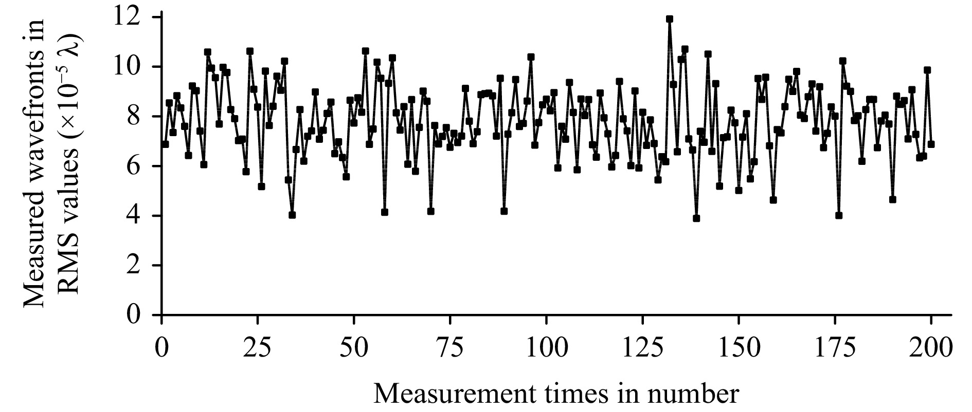
Fig. 6  Repeatability of wavefront measurement using this SHWFS.

In all cases, the residual deviations reached 8.04 × 10⁻⁵ λ (PV) and 7.94 × 10⁻⁵ λ (RMS), with a mean value of 7.81 × 10⁻⁵ λ, an order of magnitude higher than the accuracy of the wavefront measurements. It is clear that the repeatability of the results did not affect the wavefront measurement accuracy in our setup.

With removal for the three types of residual errors of the SHWFS in Section 3.3, the results in Fig. 6 show the high stability of the wavefront measurements. However, the differences in the wavefront measurements led to a large RMS value that was approximately one order of magnitude lower than the required value. Of the possible reasons for such a large repeatability RMS value, residual errors of the wavefront measurements should be considered.

Theoretically, there may be inaccuracy in the angular position for wavefront measurement with this SHWFS. As wavefront measurements were carried out using the experimental setup in Fig. 1, wavefronts generated from the pinhole had a tilt angle θ compared to the direction of the stage guiderail where the SHWFS was mounted. The change δR in the radius of the spherical wavefront induced by the tilt angle θ can be expressed by Eq. 13.

where R₀ is the radius of curvature of the spherical wavefront, with R₀ ≥ 1 m and ∂R/∂θ ≈ 10⁻² m/degree in our experimental setup. To minimize the tilt error during measurement, the uncertainty of the tilt angle should not exceed ±0.03°, leading to a residual error of 3 × 10⁻⁶ λ RMS for any wavefront measurement. Such a small residual error in wavefront measurement made a negligible contribution to the uncertainty of the wavefront measurement accuracy but introduced a certain amount of instability for mid-term measurement. Again, the residual error was approximately one order of magnitude lower than the repeatability of the wavefront measurements. This level of instability of wavefront measurements is probably a result of the residual error, air turbulence, and noise of the wavefront reconstruction procedure.

In this study, we developed and built an experimental system for calibration of an SHWFS with spherical wavefronts, in which a micrometer-scale pinhole with a diameter of 1 µm was used to generate spherical wavefronts, with residual aberrations of 1.0 × 10⁻⁴ λ RMS. The accuracy of the spherical wavefront was almost two orders of magnitude higher than that of a traditional reference source generated from a single-mode fiber, providing high-quality reference wavefronts with extremely small aberrations for SHWFS calibration.

Before used as a wavefront-measuring instrument, the SHWFS must be calibrated with high accuracy to determine the geometrical parameters of the sensor, including f, the focal length of the MLA, p, the sub-aperture size of the MLA, and s, the pixel size of the photodetector. As an approximation used in the first step of the parameter calculation procedure, a tight coupling relationship between the sub-aperture size-p and the pixel size-s was used; a modified method was used to solve for the three parameters. With only three iterations, these parameters can be determined as exact values, with convergence to acceptable accuracy.

For an SHWFS with an MLA of 128 × 128 sub-apertures in a square configuration and a focal length of 2.8 mm, spherical wavefront calibration was completed using our method. A wavefront measuring accuracy of 5.0 × 10⁻³ λ RMS was reached across the full pupil diameter of 13.8 mm. The accuracy was dependent on the residual errors induced in manufacturing and assembly of the SHWFS, which were mainly a result of imperfections in the MLA, response errors of the photodetector, and assembly errors between the MLA and photodetector.

Based on the spherical wavefront calibration, additional aberrations of the residual errors in the wavefront measurement results were analyzed in our experiments and removed by subtracting them from the measured wavefronts. The results show that the measurement accuracy of this SHWFS increased to 1.0 × 10⁻³ λ RMS with wavefront aberrations in the range of λ/4. Mid-term stability of the wavefront measurements was confirmed, with residual deviations of 8.04 × 10⁻⁵ λ PV and 7.94 × 10⁻⁵ λ RMS.

From the experiments, it was also found that the measurement accuracy of the SHWFS improved with small amplitude growth as the amplitude of the wavefront to be measured decreased. When the amplitude of the wavefront to be measured was in the range of λ/10, the measurement accuracy exceeded 2.0 × 10⁻⁴ λ, an improvement of approximately one order of magnitude. Such high accuracy meets the needs of challenging wavefront measurements such as in lithography lenses, astronomical telescope systems, and adaptive optics.

The work presented in this paper was supported by the National Key Research and Development Program of China (2021YFF0700700), the National Natural Science Foundation of China (62075235), the Youth Innovation Promotion Association of the Chinese Academy of Sciences (2019320), Entrepreneurship and Innovation Talents in Jiangsu Province (Innovation of Scientific Research Institutes), and the Jiangsu Provincial Key Research and Development Program (BE2019682).