Simulation-based design optimization of the holographic wavefront sensor in closed-loop adaptive optics

Applications such as free-space laser communications and directed energy suffer from the influence of the atmosphere. In addition to transmission losses due to absorption and scattering, these systems are particularly limited by optical turbulence. Adaptive optics (AO) systems are designed to improve the turbulence-affected pointing accuracy, data rate, resolution or focusability. This is usually done with three core components: A wavefront sensor measures the wavefront distortion. A control computer converts this measurement to a control signal.

The control signals are sent to an adaptable device such as a deformable mirror (DM) or a deformable lens to compensate for the measured wavefront deformations¹. Since the atmosphere is in motion, measurement and correction have to be performed in an open or closed loop. Depending on the turbulence strength, distance and application, the required loop rate can be a few hundred or even several thousand Hertz².

Many different technologies and types of wavefront sensors are available or under development to meet these diverse scenarios and requirements. The Shack-Hartmann wavefront sensor³, pyramid wavefront sensor⁴, curvature sensor⁵ as well as interferometric methods⁶ are widely used. Closed-loop turbulence correction was also demonstrated using a plenoptic camera⁷ as wavefront sensor and the stochastic parallel gradient descent (SPGD) algorithm for wavefront sensorless AO^8,9. Work is also being carried out on wavefront sensors based on the holographic principle¹⁰. The optical reconstruction of a hologram’s real image depends heavily on the wavefront of the reconstruction laser¹¹. It is therefore a very promising approach to use the intensity distribution of the real image to obtain information about the wavefront of the reconstructing laser.

Several methods for modal as well as zonal holographic wavefront sensing have been published. The most prominent is the modal holographic wavefront sensor (HWFS). It enables direct measurement of individual aberration modes. Core of modal HWFS is formed by two holographic gratings for each aberration of interest, which are usually multiplexed in a single hologram plate¹² or a single computer-generated hologram (CGH)¹³ to be displayed on a spatial light modulator (SLM). The sensor principle is described in detail in the next section. The advantages of this measuring method are the high achievable measuring speed (MHz bandwidths are possible) since no time-consuming calculations are needed, and the easy scalability. The same is true for the zonal HWFS¹⁴. Instead of decomposing the wavefront into individually measured aberration modes, it is sampled with a number of measuring points¹⁵. An alternative approach for holographic wavefront sensing is the use of multiplexed Fourier holograms¹⁶. With a classical Van-der-Lugt correlator¹⁷, the cross-correlation between the incident wavefront and a number of reference waves can be generated optically and the strength of aberration modes determined¹⁸.

1The HWFS enables the fastest wavefront estimation, in principle up to three orders of magnitude faster than the Shack-Hartmann wavefront sensor. However, the measurement accuracy of the sensor suffers greatly from so-called inter-modal crosstalk: different aberration modes present in the laser beam influence each other's measurements¹⁹. Several improvements have been proposed, particularly for the modal sensor, to minimize the impact of crosstalk. Neil et al²⁰. as well as Yao et al²¹. proposed a sensitivity matrix to take the crosstalk into account while Kong et al²². as well as Konwar and Boruah²³ implemented novel modifications to the wavefront sensing scheme. Dong et al. proposed avoiding the crosstalk by first closing the AO loop with the help of a second sensor of a different type^24,25. All of these approaches were able to reduce the crosstalk effect and improve the measurement accuracy to a certain degree for a limited number of modes. The HWFS has been successfully implemented in closed-loop AO systems and the high measurement speed as well as the correction capability have been proven^26-28. However, the measurements have been performed for static aberrations only and realistic optical turbulence with a high number of modes has not been addressed, yet.

In this paper, we evaluate the performance of a closed-loop AO system based on HWFS under realistic conditions: We simulate dynamic turbulence including more than 2500 modes with time-evolving amplitudes and we consider shot noise in our measurements. To reduce crosstalk effects for these challenging scenarios, we investigate a sensor optimization, which has been developed in order to increase the measurement accuracy in open-loop applications²⁹. We show that minor adaptions of the optimization procedure can improve the closed-loop AO performance even more, especially in high noise scenarios.

The modal HWFS is based on the phase biasing method^20,30: The phase of the incident beam with the unknown wavefront deformation is manipulated by adding a phase bias, as shown in Fig. 1. The bias corresponds to the aberration mode for which the HWFS is trained. The total strength of the aberration mode is the sum of the strength contained in the unknown wavefront and the strength of the bias. When the biased beam is focused, the intensity distribution in the detector plane depends on the unknown wavefront as well as on the phase bias. If the residual strength of the biased mode is zero, that is, when the bias cancels out the aberration present in the unknown wavefront, the focus of the beam is narrowest (top path in Fig. 1). In all other cases the focus is widened. The greater the residual strength of the mode, the more distributed is the light and the lower the focus intensity is in the center of the focus. Accordingly, a simple intensity measurement in a small central area around the focus (red circles on detectors in Fig. 1) gives information about the strength of the mode within the unknown wavefront³¹.

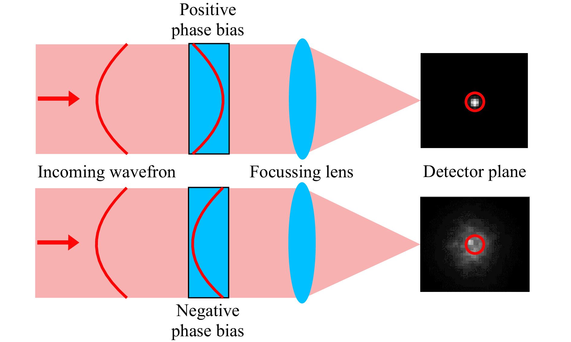
Fig. 1  Schematic representation of the phase biasing principle: A phase bias corresponding to the aberration of interest is added to the incoming wavefront. When the light is focused onto a detector, the intensity distribution depends on the residual wavefront: If the bias reduces the amplitude of the present aberration, more light is concentrated in a small central region (red circles).

However, to remove the dependency on the total intensity of the laser beam and to increase the linearity of the sensor response, a second measurement with the same bias but opposite sign is carried out (lower path in Fig. 1): Assuming a proper calibration, the contrast of the two intensity measurements gives the strength of the aberration mode sought. To measure multiple aberrations present in the wavefront, the two measurements have to be performed for each mode. By splitting the beam into two partial beams for each aberration mode and positioning a corresponding phase plate in each partial beam, all measurements can be carried out simultaneously. However, it has been proven to be very practical to generate the biased partial beams with diffraction gratings.

For the modal HWFS such diffraction gratings are produced holographically: A reference wave and an object wave are superimposed in the plane of the hologram plate. The interference pattern is recorded and acts as diffraction grating after chemical post-processing. To enable the sensor to measure aberration mode ${G_n}(x,y)$, two holograms are needed: For the first one the reference wave ${R_{n + }}$ is chosen to contain only the aberration of interest with the positive bias ${b_n}$, while the object wave ${O_{n + }}$ is a spherical wave that converges at a point $ {A_{n + }}({x_{n + }},{y_{n + }},{z_A}) $ behind the hologram plane (see Fig. 2a). For the second hologram, the reference wave ${R_{n - }}$ contains the same aberration of bias ${b_n}$, but with negative sign. The spherical object wave ${O_{n - }}$ converges at point $ {A_{n - }}({x_{n - }},{y_{n - }},{z_A}) $ (see Fig. 2b). Accordingly, the time-independent complex amplitudes of these waves in the hologram plane, that is the x/y-plane with $ z = 0 $, can be written as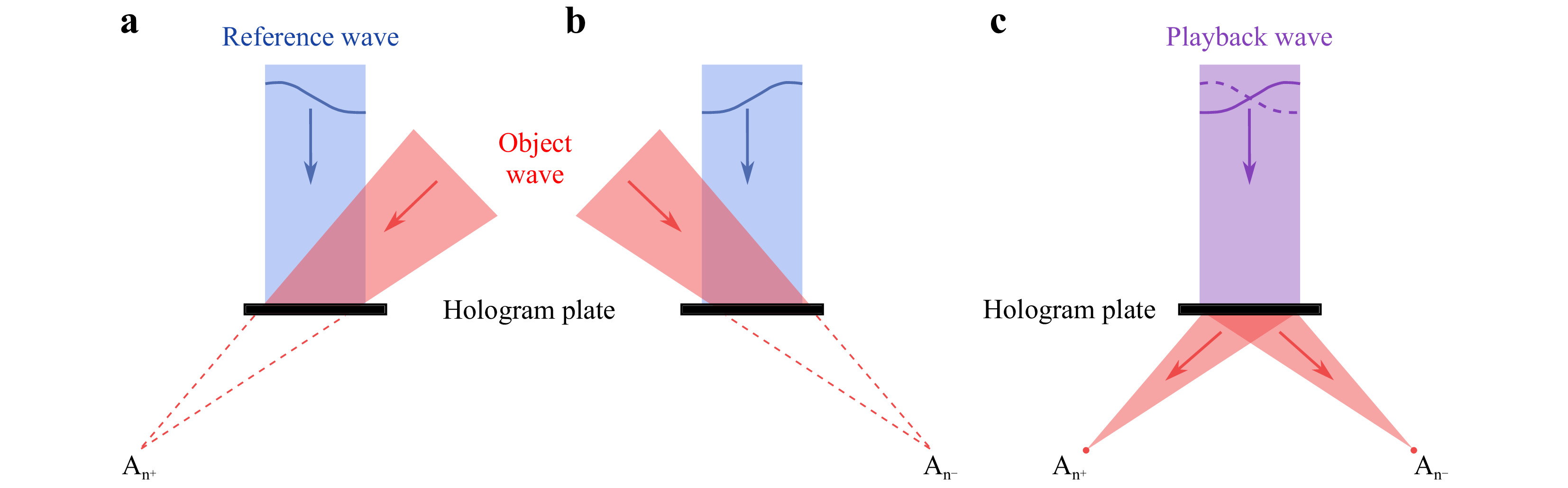

Fig. 2  Recording and reconstruction of a multiplexed hologram for holographic wavefront sensing; a first hologram with object beam converging to point A_n+ and reference beam containing the aberration of interest with positive amplitude, b second hologram with object beam converging to point A_n- and reference beam containing the aberration of interest with negative amplitude, c reconstruction of the object beams when illuminated with a playback beam.

where $k = {{2\pi } \mathord{\left/ {\vphantom {{2\pi } \lambda }} \right. } \lambda }$ is the wave number and j is the imaginary unit.

The interference patterns of ${R_{n + }}$ and ${O_{n + }}$ as well as of ${R_{n - }}$ and ${O_{n - }}$ are given by

where * denotes the complex conjugate. For the sake of readability, the spatial coordinates are omitted. The two holograms $ {H_{n + }}(x,y) $ and $ {H_{n - }}(x,y) $ are recorded with a photosensitive hologram plate. After chemical post-processing both holograms are stored as diffraction gratings. The transmission ${\tau _{n \pm }}$ of the holographic gratings is proportional to these recorded intensity distributions.

By illuminating the multiplexed hologram with a playback, or reconstruction, wave $ P(x,y) $, four waves are created for each hologram:

The first and the last terms are the zeroth diffraction orders of the playback wave, only affected in its real amplitude by $ {\left| {{R_{n \pm }}} \right|^2} $ or $ {\left| {{O_{n \pm }}} \right|^2} $. The second terms reconstruct the phase-conjugated object waves. Only the third terms are of interest for the HWFS, since they reconstruct the two object waves and with this, create two spots at the positions $ {A_{n + }} $ and $ {A_{n - }} $ (see Fig. 2c). The intensity distributions of the two reconstructed spots in the detector plane ($ z = {z_A} $) are given by

The playback wave with the wavefront $ W(x,y) $ can be represented by the weighted sum of the aberration modes as

where $ {a_i} $ is the strength or amplitude of mode ${G_i}(x,y)$. With this, the spot intensity integrated over a central detector area F can be written as

The last term in Eqs. 9,10, $ - k\sqrt {{{(x - {x_{n \pm }})}^2} + {{(y - {y_{n \pm }})}^2}} $, is responsible for the focusing of the beam in the points $ {A_{n \pm }} $. The second term, $ \left( {{a_n} \pm {b_n}} \right){G_n}(x,y) $, contains the information about the unknown amplitude $ {a_n} $ of the mode of interest. The first term, $ {\displaystyle\sum\nolimits_{ \begin{array}{l} {{ i=1}} \\[-8pt]{{ i\ne n}} \end{array}}^{\infty }}{{{a}_{i}}}{{G}_{i}}(x,y) $, describes the wavefront apart from the aberration mode of interest. If this term equals zero that means no other aberrations are present in the wavefront but the one of interest. Then the unknown amplitude $ {a_n} $ can be determined from the contrast $ {S_{{\rm{mes}},n}} $ of the two intensity measurements $ {I_{n + }} $ and $ {I_{n - }} $ as

for $ - {b_n} \leqslant {a_n} \leqslant {b_n} $. The proportionality factor $ {c_n} $ depends on the bias $ {b_n} $ and the detector size F. It can be obtained by measurements as described in a later section. If $ {a_n} = {b_n} $, the second term in Eq. 9 is canceled out and the intensity $ {I_{n + }} $ is maximum. At the same time, the intensity $ {I_{n - }} $ is minimum. If $ {a_n} = - {b_n} $, the reverse happens: The second term in Eq. 10 is canceled out and the intensity $ {I_{n - }} $ is maximum while $ {I_{n + }} $ is minimum. The relationship between $ {a_n} $ and $ {S_{{\rm{mes}},n}} $ within these limits is approximately linear.

However, if the unknown wavefront $ W(x,y) $ is distorted by atmospheric turbulence, the term $ \displaystyle\sum\nolimits_{ \begin{array}{l}{{ i=1}} \\[-8pt] {{ i\ne n}} \end{array}}^{\infty }{{{a}_{i}}}{{G}_{i}}(x,y) $ is non-zero and affects the intensity measurements. Therefore, the measurement of a particular mode is not independent of the presence of other modes. This inter-modal crosstalk causes Eq. 11 to be inaccurate. The stronger the turbulence, the less precise the measurements. This effect is particularly noticeable when measuring higher order modes. In Kolmogorov turbulence, they have on average significantly lower amplitudes than low-order modes. Accordingly, their small $ {a_n} $ is totally swamped in the phase background $\displaystyle\sum\nolimits_{ \begin{array}{l} {{i=1}} \\[-8pt] {{ i\ne n}} \end{array}}^{\infty }{{{a}_{i}}}{{G}_{i}}(x,y) $. The measurement accuracy suffers significantly. To reduce crosstalk, careful design of the modal HWFS is required²⁹. Three key design parameters can be identified in Eqs. 9,10: the modal basis $ G(x,y) $, the bias b and the detector size F. If the HWFS is designed to measure multiple aberration modes, bias and detector size have to be optimized for each aberration mode individually.

For practical and efficiency reasons, a multi-mode HWFS uses hologram multiplexing to do the beam splitting and biasing with a single diffractive optical element (DOE). All holograms, two for each mode, are recorded one after another in the same hologram plate. By illuminating this plate afterwards with the unknown wavefront, two spots for each mode are reconstructed in the detector plane. The spot pairs corresponding to a particular mode can be detected independently of the other spots. For spot detection a photodiode array or an area detector with a dedicated region of interest (ROI) for each spot can be used. The different detector sizes can be implemented by varying the sizes of the photodiodes, the chosen ROI or corresponding masks (pinholes) in front of the detector.

In the following we describe how we simulate the modal HWFS. First, we show the sensor implementation. Afterwards, we describe the simulation of HWFS-based, closed-loop AO and discuss how we generate dynamic turbulence as a sequence of correlated phase maps. Finally, we show the optimization procedure of the sensor and present adaption methods to account for its use in closed-loop configurations.

The simulation of the modal HWFS includes the holograms and the detectors. As described before, in an experimental setup, it is advantageous to implement a multi-mode sensor in a single DOE by multiplexing all sub-holograms in one multiplex-hologram. However, the multiplexing method, the number of multiplexed modes as well as the used geometry of the spots in the detector plane can influence the sensor performance³². To keep the results independent of these design-specific sources of error we treat and illuminate each sub-hologram individually and do not perform multiplexing. Accordingly, we simulate an optical setup where the incoming beam of interest is split into two partial beams per mode and each of these equal partial beams illuminates a different sub-hologram. This corresponds to the original phase biasing method.

We simulate each sub-hologram as thin phase hologram on a 256 × 256 grid. We use a circular aperture. The HWFS is coded to detect 42 modes (modes number 4 to 45 according to Noll’s indexing³³). Accordingly, the sensor consists of 2 × 42 sub-holograms. The optimal number of modes depends on the turbulence scenario, the performance of the AO system, in which the sensor is used, and the improvement goal³⁴. In order to obtain the best possible comparability of the results, we do not optimize the number of modes, but keep it constant for all simulations. The sub-holograms create 84 biased spots in the detector plane. We use Eqs. 9,10 to calculate the intensities of the spots. We optimize the bias for each mode individually as we will discuss in a later section. We simulate each spot in the detector plane with 256 × 256 pixels. The pixel scale corresponds to $ \lambda /2D $, D is the aperture of the optical system and $ \lambda = 1550 $ nm the wavelength of the laser beam. We normalize the spots to have a total power of one by dividing each pixel value by the sum of all pixel values. Afterwards, we multiply each pixel by the number of signal photons focused into the spot to get the number of photons per detector pixel. To determine $ {I_{n + }} $ and $ {I_{n - }} $, all photons inside the particular ROI are summed for each spot. We optimize the ROI for each mode individually as described in a later section. We choose the unit of the ROI to be $ \lambda /D $. Hence, the results are independent of specific detector designs and dimensions.

In our simulations, we consider nine signal-to-noise ratio (SNR) scenarios. We implement the different SNRs by limiting the average number of signal photons per spot and introducing shot noise³⁵. Shot noise can be modeled as a Poisson process; its variance equals the average number of photons $ {N_{Ph}} $ and the SNR is given by

For each scenario, the average number of photons and the corresponding SNR is listed in Table 1. The first scenario does not include noise. We assume that the diffraction efficiency is identical for all sub-holograms and that the average number of signal photons is equal for all spots. However, the number of photons inside the specific ROIs differs depending on the particular bias and the aberrations present in the beam.

To generate the noisy signal, we consider shot noise only. Other sources of noise, such as readout noise, depend on the detector. Especially the number of pixels is crucial to determine the total amount of noise in the presence of readout noise. Accordingly, it would be necessary to perform the simulations for a particular detector. In contrast, shot noise can be treated independently of most of the specifications of the detector (we assume a quantum efficiency of 100% and do not consider the dynamic range of the detector). The noise is applied by replacing the photon sums $ {I_{n + }} $ and $ {I_{n - }} $ with a Poisson random draw based on mean value given by these photon sums. Afterwards we compute their weighted contrast to determine the amplitude of the particular mode (Eq. 11). The needed calibration factor $ {c_n} $ is obtained during the optimization process, as described in a later section.

We implement the HWFS based on two different modal bases: Zernike modes denoted with Z and Karhunen-Loève modes denoted with K. The advantage of Zernike modes is their simple analytic expression. They are widely used in AO and are the basis of choice in nearly all publications about holographic wavefront sensing. However, Zernike modes are not the best choice to describe Kolmogorov turbulence statistics³⁴. Some Zernike modes are correlated which involves redundancy when representing turbulence. Karhunen-Loève modes are designed to remove this redundancy. They can be expressed as linear combination of Zernike modes

with the coefficients $ {u_{jk}} $^36,37. All Karhunen-Loève modes are statistically independent. Hence, if a finite number of modes is used to represent a wavefront, Karhunen-Loève modes contain the maximum amount of information. If the same number of Zernike and Karhunen-Loève modes are perfectly corrected by an ideal AO system, the residual phase variance of the wavefront is lower for the Karhunen-Loève-based system³⁸. We will compare HWFS based on Karhunen-Loève modes and Zernike modes. The interested reader can find a detailed description of how we calculate the Karhunen-Lòeve modes in Ref.⁹ and a comparison of the first 50 Zernike and Karhunen-Karhunen-Loève modes in Fig. 3 of Ref. 39.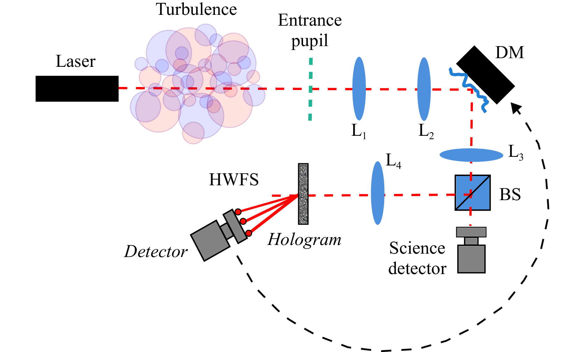

Fig. 3  Principle design of a basic post-compensation closed-loop AO system. The entrance pupil is imaged with lenses L₁ and L₂ in the DM plane and with lenses L₃ and L₄ in the hologram plane. The beamsplitter BS directs some light to the wavefront sensor and transmits most of it to be focused on the science detector. Wavefront sensor signal is used as control signal for the DM.

We simulate a basic closed-loop AO system based on modal HWFS. We assume post-compensation AO with wavefront measurement and correction at the receiver side, as it is widely used in astronomical and laser communications applications. Nevertheless, the results can also be transferred to a pre-compensation scheme, where wavefront measurement and correction are performed at the transmitter. Pre-compensation is of special relevance for directed energy applications with non-cooperative targets⁴⁰. The principle of our post-compensation AO system is illustrated in Fig. 3: After passing the atmospheric turbulence, the laser light is reflected by the DM to be focused onto a detector. In a real AO system, this detector is the receiver for scientific measurements. We use this detector to monitor the AO performance. In the following, we refer to it as the science detector. Part of the light is directed to the HWFS by a beam splitter (BS). The entrance pupil of the optical system, the DM and the hologram plate are conjugated planes. The light is diffracted at the multiplexed holographic grating into the spots. The spots are sensed by the HWFS detector and the amplitudes of the aberration modes are determined. The wavefront, approximated by the HWFS measurement, is composed by summing the modes multiplied by the measured amplitudes. To correct for this distorted wavefront, it is conjugated, multiplied by the AO gain and passed to the DM as control signal to reshape its reflective surface accordingly. Measurement and correction are performed in a loop with the AO bandwidth to adapt to the temporally-evolving turbulence. In a closed-loop system, no absolute measurement of the wavefront at the entrance pupil is performed, instead the wavefront sensor measures the residual wavefront distortion after the light has passed the DM. As control scheme we assume a traditional pure integrator, where the measured residual wavefront $ W_{}^{res} $ is multiplied by the gain g and subtracted from the prior surface shape of the DM $ W_{m - 1}^{DM} $ to obtain the desired new shape of the DM $ W_m^{DM} $⁴¹.

where the AO correction step m.

To simulate the effect of atmospheric turbulence, we use pupil-plane phase maps. To represent dynamic turbulence, the phase maps are generated as a correlated sequence.

Wavefronts propagating through the atmosphere are usually affected by several turbulence layers moving at different speeds. This leads to wavefront deforming over time, so-called “wavefront boiling”⁴². Hence, for a realistic simulation of the wavefront dynamics, a turbulence profile, represented by the refractive index structure constant $ {C_N}^2 $, as well as a wind speed profile along the beam path is needed. We created a $ {C_N}^2 $ profile based on models and measurements by Montoya et al⁴³. and Zhang and Wang⁴⁴ and the wind speed profile from García-Lorenzo et al⁴⁵. Both profiles apply to Canary Islands during daytime. The profiles are discretized in nine layers. The heights and the median wind speeds of each layer are listed in Table 2.

We represent each of the nine layers by a single phase strip. To fill the strips with phase values according to the turbulence profile of the individual layer, we use the FFT-based method of McGlamery⁴⁶. The layers are virtually aligned above the entrance pupil of our AO system. We define the turbulence sampling frequency to be 4 kHz. We translate the phase strips according to the average wind speed of the corresponding layer (Table 2) from right to left. Fig. 4 shows the procedure for four phase strips as an example. The lengths of the yellow arrows represent the median wind speed of each layer. After the translation, we crop the 256 × 256 pixel region above the pupil of each phase strip (red boxes in Fig. 4) and sum their phase values to obtain the phase map in the pupil-plane. After 4000 translations we obtain a sequence of 4000 correlated phase maps representing in total one second of dynamic turbulence. We generate phase map sequences for the normalized turbulence strengths $ {D \mathord{\left/ {\vphantom {D {{r_0}}}} \right. } {{r_0}}} = 4 $ to $ {D \mathord{\left/ {\vphantom {D {{r_0}}}} \right. } {{r_0}}} = 20 $, where D is the aperture and $ {r_0} $ is the Fried parameter for plane wave.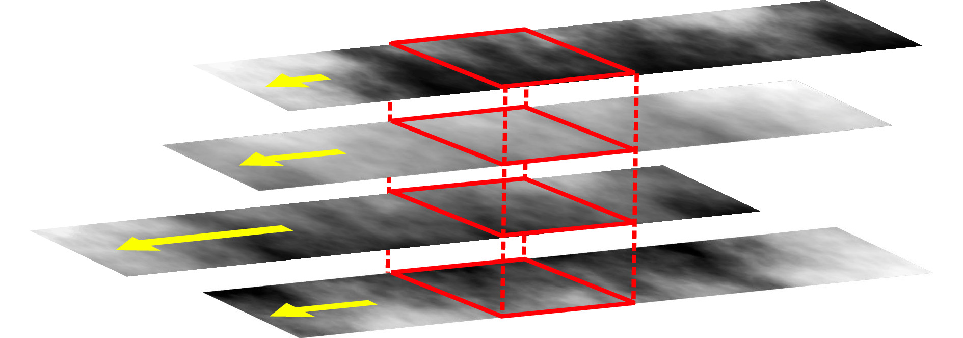

Fig. 4  To simulate a phase map sequence to represent dynamic turbulence, each turbulence layer is represented by a phase strip. Phase strips are translated according to the median wind speed of their layer (represented by yellow arrow) and the phase values inside the red boxes are added to obtain the pupil-plane phase map.

In our AO simulations we assume perfect tip and tilt correction. Thus, we remove global tip and tilt in all phase maps.

We simulate the closed-loop correction of this dynamic turbulence as sketched in Fig. 5. The top row shows the phase maps applied to the system at its sample bandwidth of 4 kHz. The bottom row shows the measurements of the HWFS as weighted sum of the 42 detected modes. The second row represents the shape of the DM. Before the first measurement, the surface is flat. Afterwards it is shaped according to the HWFS measurement. We assume the DM to be ideal and to assume the prescribed shape perfectly. The shape of the DM is updated only after a HWFS measurement. Since the AO bandwidth is lower than the bandwidth with which we sample the dynamic atmosphere (in the sketched example three times smaller), measurement and correction are not performed for each phase map. That means that the turbulence evolves between the AO iterations while the DM surface remains unchanged. To monitor the performance of the AO system, we simulate the point spread function (PSF) of the focused beam in the plane of the science detector with 256x256 pixels of pixel size $ \lambda /2D $. This corresponds to Nyquist sampling of a diffraction limited PSF and is obtained by zero padding of the wavefront⁴⁷. A cross-section of the PSFs is displayed in the third row of Fig. 5 in blue. The red line represents the Strehl ratio over time. We use the Strehl ratio as quality metric and calculate it as peak of the PSF divided by the peak of the diffraction-limited PSF⁴⁸. Both PSFs are normalized to have the same total power.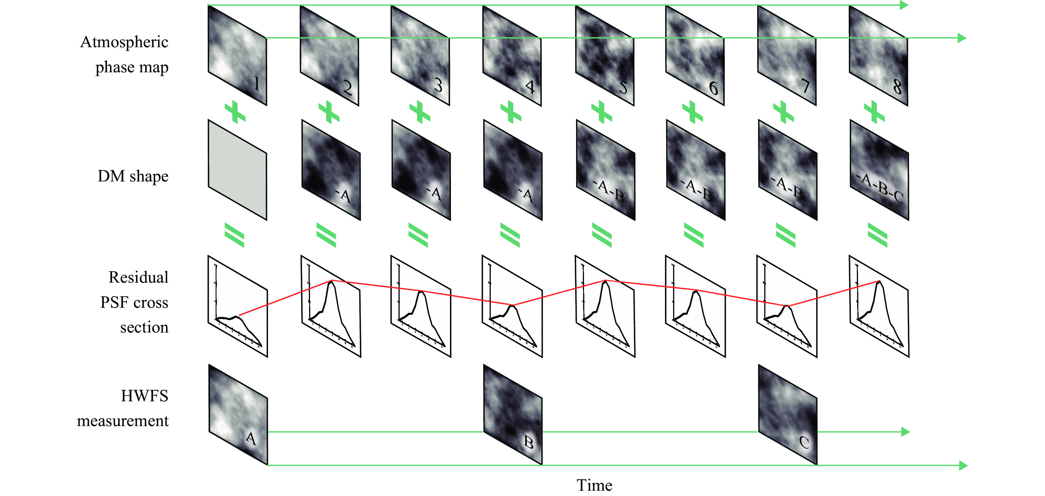

Fig. 5  Depiction of HWFS-based AO simulation with dynamic turbulence. Top row: atmospheric phase map sequence is applied to the system at its sample rate (4 kHz). Second row: DM shape is updated after each HWFS measurement. The measured residual wavefront is subtracted from the current DM shape. Third row: the corrected wavefront is focused onto the science detector. The cross-section of the PSF is shown in blue. Red line represents the Strehl ratio over time. Bottom row: HWFS measurement of the residual wavefront, performed at the AO bandwidth (AO bandwidth < turbulence sample rate).

Phase bias and ROI are key design parameters of the modal HWFS. The combination of the two has a major impact on the occurrence of inter-modal crosstalk. Accordingly, a proper choice of bias and ROI can improve the measurement accuracy significantly. The best combination, however, differs for different modal bases, individual modes and turbulence strengths. To determine the optimal combination of bias and ROI, we use an optimization method that aims to find the parameters with the weakest crosstalk²⁹. The workflow of the optimization procedure is shown in Fig. 6. The optimization has to be performed for each turbulence strength ($ {D \mathord{\left/ {\vphantom {D {{r_0}}}} \right. } {{r_0}}} $) individually and on a mode-by-mode basis.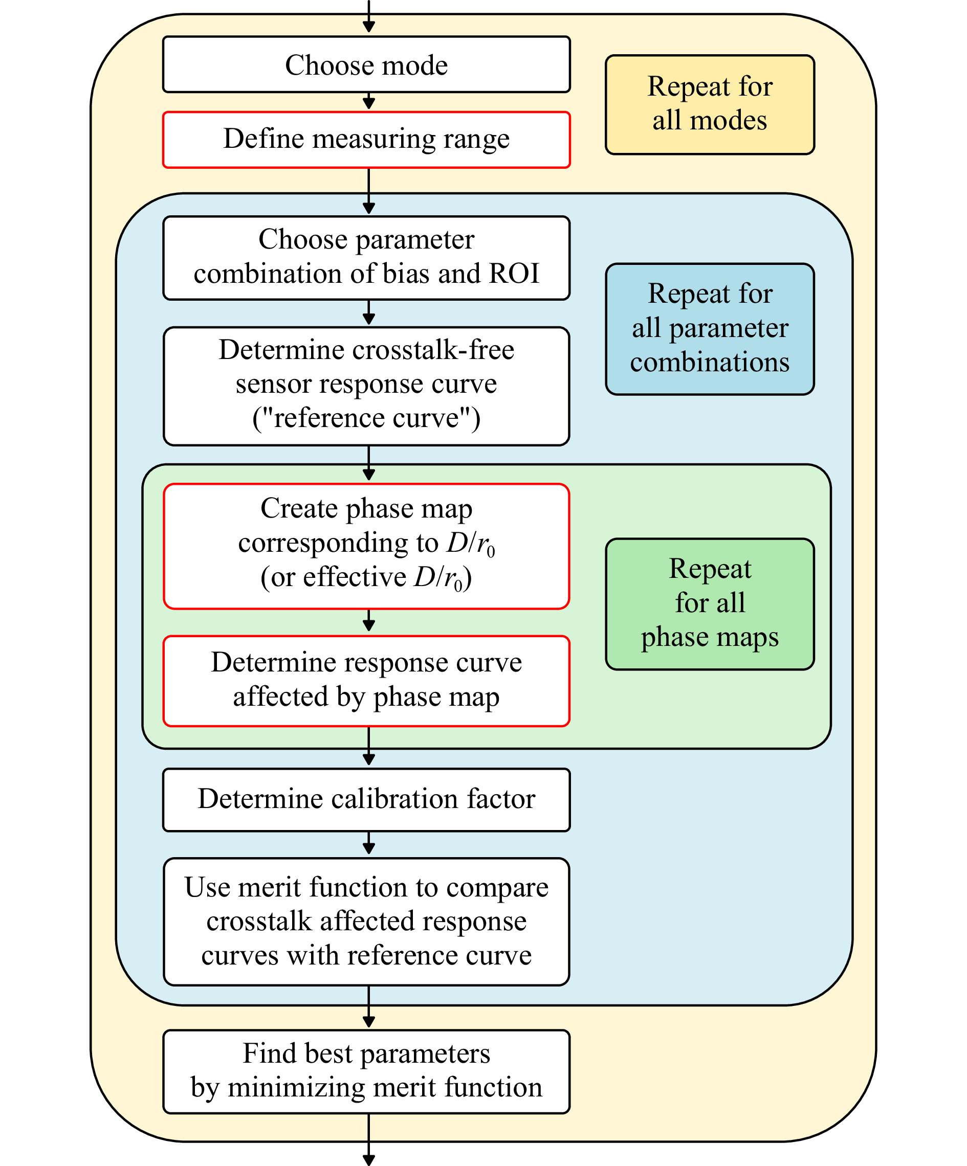

Fig. 6  Workflow of the optimization procedure for finding the best combination of bias and ROI to reduce crosstalk effects.

It makes sense that the measuring range is based on the expected range of variability of the mode of interest $ {G_n}(x,y) $ for the given turbulence strength. We choose the range to be three times the modes’ standard deviation $ {\sigma _n} $ in Kolmogorov turbulence³³. For all relevant combinations p of bias $ {b_n} $ and ROI $ {F_n} $, a crosstalk-free sensor response curve $ {S_{{\rm{ref}},n,p}} $ is determined as a reference. The sensor response curve is the result of M measurements (Eq. 11), whereby the wavefront $ W(x,y) $ of the playback beam contains the mode of interest $ {G_n}(x,y) $ only. The amplitude $ {a_n} $ of this mode is successively increased for each of the M measurements to cover the entire measuring range, while $ {a_{i \ne n}} = 0 $ (see Eq. 8). Accordingly, the term $ \displaystyle\sum\nolimits_{i \ne n}^\infty {{a_i}} {G_i}(x,y) $ vanishes in Eqs. 9,10 and the reference response curve cannot be affected by crosstalk. The dashed black curve in Fig. 7a shows an example of a reference response curve.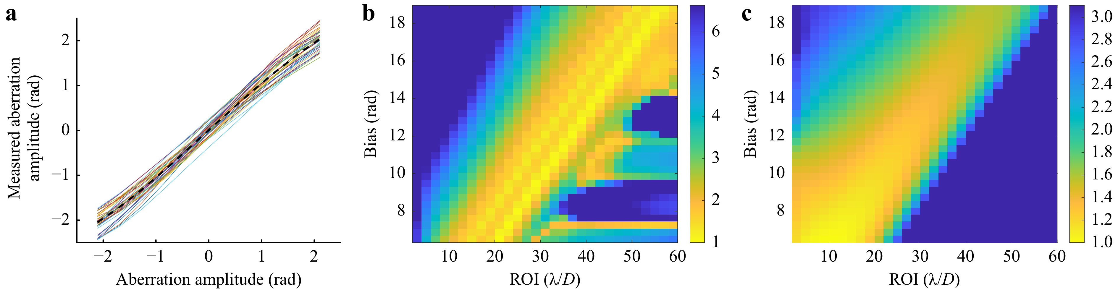

Fig. 7  a Optimization results of HWFS to measure Karhunen-Loève mode 4 at turbulence strength of D/r₀=10; dashed black curve: crosstalk-free reference sensor response; solid colored curves: crosstalk-affected response curves, obtained from different independent phase maps representing D/r₀=10; b J-map: merit function for bias and ROI combinations, values greater than the median are set to the median; c c-map: calibration factors for bias and ROI combinations, values greater than the median are set to the median.

In the next step, a response curve $ {S_{{\rm{mes}},n,p}} $ is measured for a playback beam that is distorted by realistic atmospheric turbulence. We simulate the distorted wavefront $ W(x,y) $ as the weighted sum of 2555 Zernike modes. We exclude the first three modes, piston, tip and tilt, from this phase map. The weighting factors are normally distributed random variables. Their standard deviation $ {\sigma _n} $ is obtained with the turbulence strength and the diagonal elements $ {c_{nn}} $ of the covariance matrix of Zernike modes in Kolmogorov turbulence⁴⁹:

The weighting factor of the mode of interest is not set as random number like for the other modes. Instead, we increase $ {a_n} $ successively for each of the M measurements within the measurement range to determine the response curve. The obtained response curve differs from the reference curve, since the high number of modes present in the phase map creates crosstalk. For stronger turbulence as well as for modes of higher order, the crosstalk increases and the curve deviates more from the reference. However, the measurement of a single crosstalk-affected response curve alone is not sufficient, since the amplitudes of the aberrations are random and the crosstalk can therefore vary greatly. We repeat the measurements k times to obtain k crosstalk-affected response curves. For each response curve a different phase map is created and applied. The phase maps are independent and uncorrelated. For sensor calibration, we calculate the mean of all k response curves to obtain the average response curve. We approximate the proportionality or calibration factor $ {c_n} $ (see Eq. 11) of the HWFS as the reciprocal slope of a linear fit to the average response curve. The smaller the calibration factor, the higher the sensitivity of the sensor. The colored curves in Fig. 7a display 40 calibrated crosstalk-affected response curves for mode 4 (defocus).

To compare the crosstalk-affected response curves with the reference curve, we calculate the merit function $ {J_{n,p}} $ for the current mode and parameter combination as

where the symbol $\left\langle {\;\;} \right\rangle $ denotes sample averaging over the k measurements. For the simulations presented in this paper we set $ k = 40 $ and $ M = 11 $. The first term of the merit function J calculates the deviation of the average response curve from the reference curve. The second term determines the deviation of each of the k crosstalk-affected response curves from the reference. Smaller J means that the crosstalk-affected curves are more similar to the reference and with this that the crosstalk is smaller.

After repeating this procedure for all relevant combinations of bias and ROI, we can summarize the results in two maps: The J-map contains the results of the merit function for all parameter combinations and the c-map contains the determined calibration factors for the same combinations. A normalized J-map is shown in Fig. 7b, the corresponding normalized c-map in Fig. 7c. Normalization is performed by dividing J and c by their smallest value. Bias is plotted on the y-axis, ROI on the x-axis. Outliers are suppressed by replacing all values that are greater than the median with the median (blue color). A small value (yellow color) in the J-map means that the crosstalk is comparatively low for this combination and a small value in the c-map means that the sensitivity of the sensor is comparatively high for this combination. We obtain individual J- and c-maps for different modes and turbulence strengths.

To find the optimal HWFS design, i.e. the best combination of bias and ROI, we minimize the merit function. Specifications of the used detector like dynamic range or scenarios in the starved-photon regime might limit the acceptable sensitivity of the HWFS. In that case we can take the c-map into account to exclude combinations that do not fulfill the sensitivity requirements.

It has been proven that choosing a sensor design based on this optimization procedure increases the measurement accuracy of the modal HWFS significantly²⁹. The sensor is designed for a certain turbulence strength ($ {D \mathord{\left/ {\vphantom {D {{r_0}}}} \right. } {{r_0}}} $) and takes into account the turbulence statistics and the expected amplitudes of the modes. Using the sensor in turbulence scenarios that it was not optimized for will most likely still give good results, albeit not as good as when the sensor is used in conditions it was designed for. The same can be expected when implementing the optimized HWFS in a closed-loop AO system. After closing the loop and starting the correction, the residual amplitudes of the measured modes, and with this the sizes of the spots, are reduced. As a consequence, bias and ROI are no longer optimal for the new, residual conditions. Additionally, the crosstalk that emanates from the corrected modes is reduced. To account for changing conditions during closed-loop operation, we propose to modify the optimization procedure. The modified steps are outlined in red in the workflow chart (Fig. 6).

1. The sensor is not optimized for the turbulence strength $ {D \mathord{\left/ {\vphantom {D {{r_0}}}} \right. } {{r_0}}} $ of the expected turbulence scenario, but for an effective $ {D \mathord{\left/ {\vphantom {D {{r_0}}}} \right. } {{r_0}}} $ that corresponds to the conditions during closed-loop operations. Thus, phase maps to represent the turbulence strength have to be created for the effective $ {D \mathord{\left/ {\vphantom {D {{r_0}}}} \right. } {{r_0}}} $.

2. With smaller residual amplitudes of the modes, the measuring range can be reduced to increase the accuracy in that smaller region.

3. The expected SNR and photon numbers are considered by applying both to the response curve measurements.

First, we present the performance analysis of the modal HWFS in closed-loop operation in realistic turbulence. We compare results from Zernike- and Karhunen-Loève-based AO systems with and without optimization. We then show that adapting the sensor optimization to the expected SNR scenario and to closed-loop operation increases its performance. Finally, we propose the use of a multi-ROI HWFS to improve the measurement accuracy of the sensor in closed-loop operation.

To evaluate the performance of an AO-system based on HWFS, we simulate closed loop operation as described before. We use the Strehl ratio of the PSF on the science detector as performance metric. The results for the turbulence strength $ {D \mathord{\left/ {\vphantom {D {{r_0}}}} \right. } {{r_0}}} = 10 $ are shown in Fig. 8. The HWFS is coded to measure the modes 4 to 50. We set the AO bandwidth to 2 kHz and the AO gain to 0.3. Fig. 8a presents the results of the Zernike-based system, Fig. 8b of the Karhunen-Loève-based system. The x-axes show the time, sampled with 4000 correlated phase maps of dynamic turbulence. The y-axes show the Strehl ratio. The solid lines represent the instantaneous Strehl ratios, while the dashed lines of the corresponding color visualize their mean value. The red curves in both panels show the Strehl ratio if no AO correction is performed. Since the same turbulence sequence is used, the two Strehl ratios without AO are identical. The black curves represent the AO performance with perfect HWFS measurement, i.e. without measurement errors. This is the maximum the system can achieve for the given AO bandwidth, gain and number of modes. Due to the higher variances of low-order Karhunen-Loève modes than their Zernike counterparts and their statistic independency, the mean Strehl ratio of the perfect Karhunen-Loève-based system (black dashed line in panel b) is higher than the one of the perfect Zernike-based system (black dashed line in panel a). Karhunen-Loève-based AO is capable of achieving higher Strehl ratios. The blue curves correspond to the use of HWFS without optimization. Instead of performing the optimization method to find the best combination of bias and ROI, we set the two parameters according to simple, common-sense guidelines: We chose the bias to define the measurement range and set it to $ 3\sigma $ of the modes. We keep the ROI relatively small to maximize the sensor sensitivity and set it to five times the size of the diffraction limited PSF. Compared to the case of no correction (red curves), a clear improvement can be seen for both bases. While the results in open-loop operation suffer from the limited measurement accuracy due to crosstalk²⁹, the results in closed-loop operation are less affected. The reason is that by decreasing the amplitudes of the modes during operation, their crosstalk to other modes decreases as well. Nonetheless, there is still potential for improvement compared to the case of perfect correction. The magenta curves show the performance of the optimized HWFSs. Here we chose bias and ROI according to the optimization results for the specific $ {D \mathord{\left/ {\vphantom {D {{r_0}}}} \right. } {{r_0}}} $. This optimization leads to significant improvement of the performance. For the Zernike sensor the mean Strehl ratio is increased from 0.31 without optimization to 0.49 with optimization. For the Karhunen-Loève sensor the mean Strehl ratio is increased even more from 0.37 to 0.6. When comparing the results of both modal bases with optimization (magenta curves in panel a and b), it can be seen that the Karhunen-Loève-based AO achieves a higher Strehl ratio. Additionally, the difference between optimized HWFS AO and perfect HWFS AO is smaller. This shows that the optimization is more efficient for Karhunen-Loève modes. Accordingly, this modal basis is the best choice for HWFS in closed-loop operation.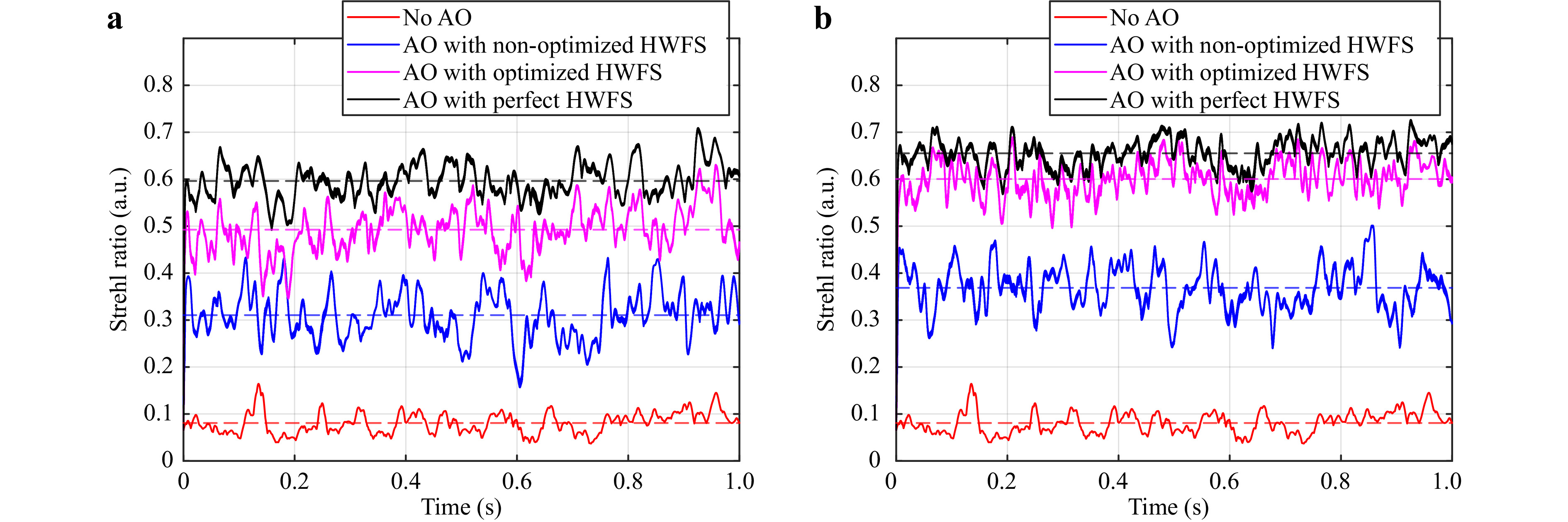

Fig. 8  Strehl ratio over time for closed-loop AO with Zernike-based HWFS a and Karhunen-Lòeve-based HWFS b. The turbulence strength is D/r₀ = 10, the AO bandwidth is 2 kHz and the AO gain is 0.3. 45 modes are measured and corrected. Dashed lines: mean values of the instantaneous Strehl ratios.

Although the optimized HWFS achieves very good results in closed-loop operation, these are likely not the best possible results. The measurement environment for the HWFS changes during closed-loop operation: the variances of the modes decrease as well as the spot sizes. Hence, the conditions differ from those during the optimization process. Especially in challenging scenarios like high $ {D \mathord{\left/ {\vphantom {D {{r_0}}}} \right. } {{r_0}}} $ or poor SNR, we expect that there is potential for further improvement. As described before, we adapt the optimization method to account for the closed-loop operation. In order to simplify the distinction, we refer to the original optimization as “classic optimization” and to the adapted optimization as “modified optimization”.

Fig. 9 shows the measurement error of Karhunen-Loève-based HWFSs as a function of SNR. We use the HWFSs to measure the amplitudes of 42 modes in 100 independent, uncorrelated phase maps. The phase maps represent the turbulence strength of interest. To define the accuracy, we do not look at the absolute measurement error but the measurement error relative to the standard deviation $ {\sigma _n} $ of the measured mode. Therefore, we divide the root mean square (RMS) error of these 100 amplitude measurements by $ {\sigma _n} $ and average over all modes. Multiplied by 100 the cost function E is given in percent by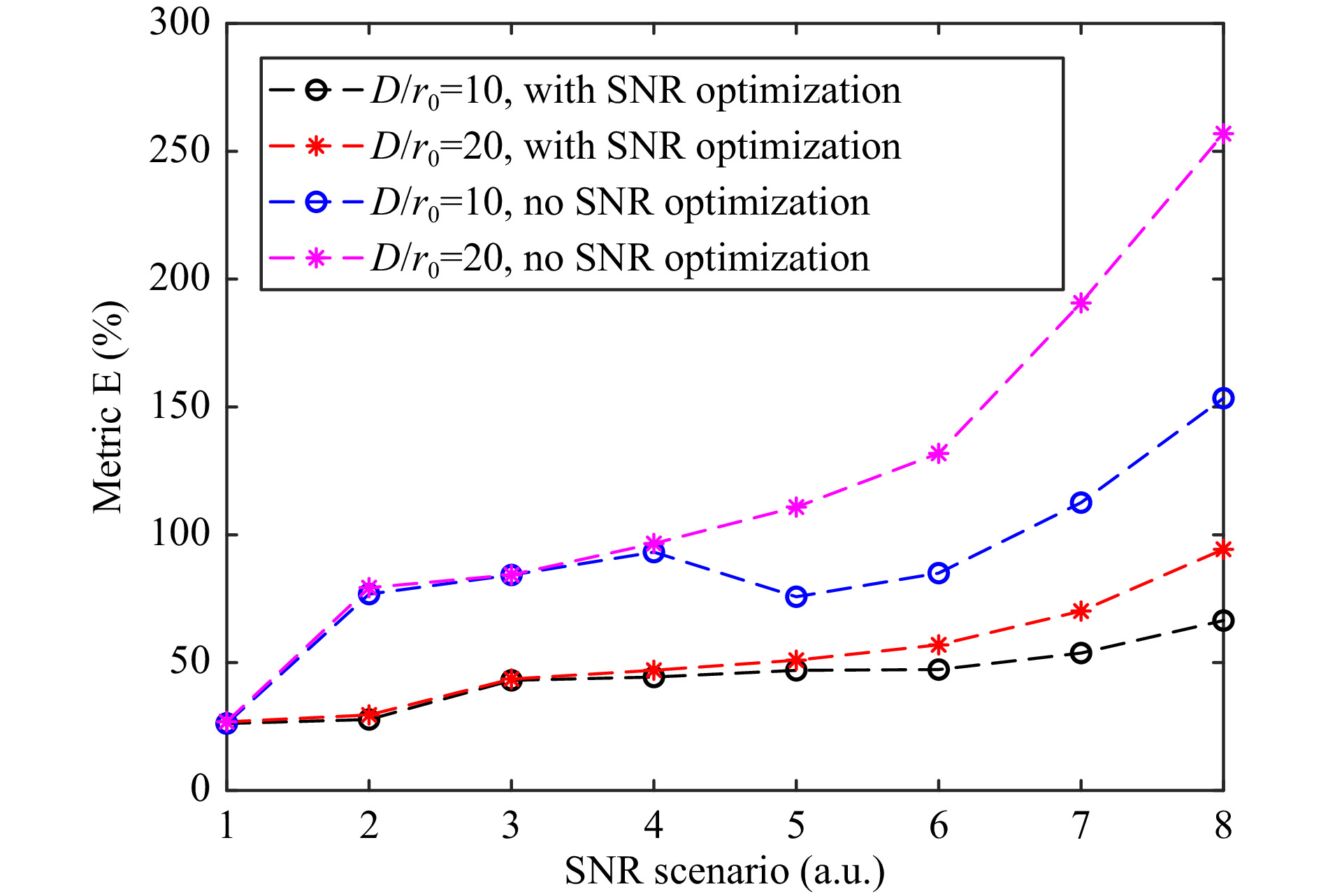

Fig. 9  Cost function E as function of SNR scenario for classic optimization (blue and magenta curve) and modified optimization (black and red curve). HWFS is coded to measure 42 Karhunen-Loève modes. Results are based on 100 measurements of independent, static phase maps corresponding to D/r₀=10 (black and blue curve) and D/r₀=20 (red and magenta curve).

where N is the number of the highest mode, M the number of independent phase screens, $ {U_{{\rm{mes}},n,m}} $ the measured amplitude and $ {U_{{\rm{truth}},n,m}} $ the ground truth of the nth mode at the mth phase map.

The higher the cost function, the less accurate the measurements are. The blue curve in Fig. 9 shows the cost function (metric E) of a classically optimized HWFS designed for $ {D \mathord{\left/ {\vphantom {D {{r_0}}}} \right. } {{r_0}}} = 10 $ and measuring at $ {D \mathord{\left/ {\vphantom {D {{r_0}}}} \right. } {{r_0}}} = 10 $. The optimization did not take SNR into account. Accordingly, the optimal bias and ROI for SNR scenario 1 (no noise present) is used for all SNR scenarios. The magenta curve shows the error of a HWFS measuring at $ {D \mathord{\left/ {\vphantom {D {{r_0}}}} \right. } {{r_0}}} = 20 $, designed for this turbulence strength but without SNR optimization. The black and the red curves correspond to the metric E of HWFSs where we took the SNR during the optimization into account: Bias and ROI are optimized for each SNR independently. For SNR scenario 1 the displayed metric is about 25% for all four sensors, i.e. the average measurement error is about 25% of the modes’ standard deviation. For the classically optimized sensors the measurement error increases sharply as the signal-to-noise ratio decreases. A reliable, reproducible measurement hardly seems possible in demanding scenarios. The optimal parameters for noiseless measurements are not the best choice for noisy measurements. Modifying the process to optimize each scenario independently increases the accuracy significantly.

To account for the changing conditions during closed-loop operation, we do not optimize for the initial turbulence strength, which is given by the turbulence scenario, but for an effective turbulence strength given by the performance of the locked-in AO system. To define the effective turbulence strength, we assume an AO system based on a perfect HWFS and analyze the residual amplitudes of the modes during the closed-loop operation. Since with ideal HWFS no measurement errors occur and the perfectly measured amplitudes are corrected perfectly, these residual amplitudes are the lowest that can be achieved. However, because of the limited AO bandwidth and an AO gain smaller than 1, the residual amplitudes are nonzero. Fig. 10a shows results for closed-loop measurements with perfect HWFS with different gain and bandwidth combinations for $ {D \mathord{\left/ {\vphantom {D {{r_0}}}} \right. } {{r_0}}} = 10 $. The presented relative mean residual amplitudes RMRA_n are defined for each mode number n as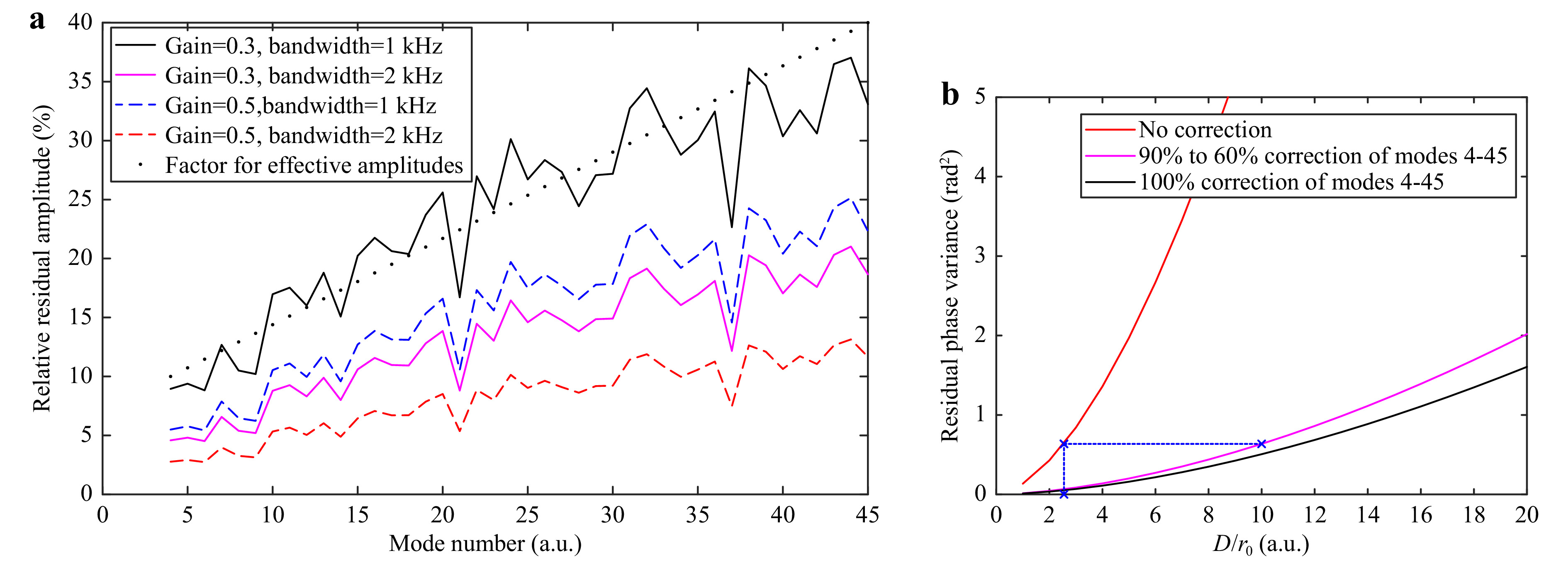

Fig. 10  a Relative residual mean amplitude of closed-loop AO with perfect HWFS at D/r₀=10 for different gain and bandwidth combinations. The black dots correspond to a linear fit applied to the black graph. b Pupil-averaged residual phase variance as function of D/r₀.

where M is the number of measured correlated phase maps of the sequence and $ {a_{{\rm{res}},n,m}} $ is the measured residual amplitude of the nth mode at the mth phase map. In Eq. 18 the absolute values of all residual amplitudes of the sequence are averaged and divided by the standard deviation of the corresponding mode. Because higher order modes suffer more from crosstalk, the relative mean residual amplitudes increase with increasing mode number. We see that a perfect AO system with a gain of 0.3 and a bandwidth of 1 kHz at $ {D \mathord{\left/ {\vphantom {D {{r_0}}}} \right. } {{r_0}}} = 10 $ can reduce the amplitudes to roughly 10% to 40% of $ {\sigma _n} $ (solid black curve). We use this information to determine our expected effective turbulence strength after closing the loop. We define a correction factor $ {f_n} $ ascending from 10% to 40% for each mode (shown as black dots in Fig. 10a). We use these factors to create phase maps for the effective turbulence strength: we generate phase maps for the initial turbulence strength $ {D \mathord{\left/ {\vphantom {D {{r_0}}}} \right. } {{r_0}}} $ but multiply the amplitudes of the modes that we want to measure and correct by the corresponding factor $ {f_n} $. Additionally, we reduce the measurement range we want to optimize for from $ 3{\sigma _n} $ to $ 2{\sigma _n} $. This modified optimization is referred to as “adapting the initial $ {D \mathord{\left/ {\vphantom {D {{r_0}}}} \right. } {{r_0}}} $”.

An alternative approach to generate an effective $ {D \mathord{\left/ {\vphantom {D {{r_0}}}} \right. } {{r_0}}} $ is to find a $ {D \mathord{\left/ {\vphantom {D {{r_0}}}} \right. } {{r_0}}} $ (lower than the initial one) by matching the phase variance. The pupil-averaged phase variance $ \left\langle {{\varepsilon ^2}} \right\rangle $ can be calculated as the sum of the variances of all modes. With Eq. 15 and the assumption that piston is ignored and tip and tilt are perfectly corrected, this can be written as⁵⁰

where N is the index of the highest mode, that is measured and corrected. The phase variance is split in two terms: the first contains the modes that can be corrected by the AO system and the second includes all other modes. The second term is approximated by an asymptotic formula found by Noll³³. In Fig. 10b the residual phase variance is shown as function of $ {D \mathord{\left/ {\vphantom {D {{r_0}}}} \right. } {{r_0}}} $. The red curve shows the residual phase variance when no AO correction is performed, i.e. when we set the correction factor $ {f_n} = 1 $ for all modes. This corresponds to the phase variance of the initial, uncorrected turbulence strength.

The black curve represents a perfect correction of the first N modes, i.e. when we set the correction factor $ {f_n} = 0 $ for all modes. To create the magenta curve, we chose an ascending correction factor, increasing from 0.1 to 0.4 with increasing mode number. Thus, the curve represents a partial correction of the modes, corresponding to the residual amplitudes we determined for AO with perfect Karhunen-Loève-based HWFS, gain of 0.3 and bandwidth of 1 kHz at $ {D \mathord{\left/ {\vphantom {D {{r_0}}}} \right. } {{r_0}}} = 10 $. As illustrated with the blue dotted lines, an uncorrected turbulence strength of $ {D \mathord{\left/ {\vphantom {D {{r_0}}}} \right. } {{r_0}}} = 3 $ has roughly the same phase variance as the partially corrected turbulence strength of $ {D \mathord{\left/ {\vphantom {D {{r_0}}}} \right. } {{r_0}}} = 10 $. Hence, we can define $ {D \mathord{\left/ {\vphantom {D {{r_0}}}} \right. } {{r_0}}} = 3 $ as the effective turbulence strength for closed-loop operation at $ {D \mathord{\left/ {\vphantom {D {{r_0}}}} \right. } {{r_0}}} = 10 $. Effective turbulence strengths can be found for other turbulence scenarios accordingly. The optimization is performed for the effective $ {D \mathord{\left/ {\vphantom {D {{r_0}}}} \right. } {{r_0}}} $ instead of the initial one. This modified optimization is referred to as “changing to different $ {D \mathord{\left/ {\vphantom {D {{r_0}}}} \right. } {{r_0}}} $”.

In Fig. 11 the classic optimization and the two modified optimizations, i.e. adapting and changing $ {D \mathord{\left/ {\vphantom {D {{r_0}}}} \right. } {{r_0}}} $ while considering SNR conditions, are compared. The optimized HWFSs were used to measure 42 Karhunen-Loève modes in a closed-loop AO system with a gain of 0.3 and a bandwidth of 1 kHz. The mean Strehl ratio of the PSF on the science detector is shown for the SNR scenarios 1, 4 and 7. Results are given for the turbulence strengths $ {D \mathord{\left/ {\vphantom {D {{r_0}}}} \right. } {{r_0}}} = 10 $ (dashed lines) and $ {D \mathord{\left/ {\vphantom {D {{r_0}}}} \right. } {{r_0}}} = 20 $ (dotted lines). HWFSs with classic optimization are plotted in red, with modified optimization based on adapting the $ {D \mathord{\left/ {\vphantom {D {{r_0}}}} \right. } {{r_0}}} $ in black and with modified optimization based on changing the $ {D \mathord{\left/ {\vphantom {D {{r_0}}}} \right. } {{r_0}}} $ (changing to $ {D \mathord{\left/ {\vphantom {D {{r_0}}}} \right. } {{r_0}}} = 3 $ for $ {D \mathord{\left/ {\vphantom {D {{r_0}}}} \right. } {{r_0}}} = 10 $ scenario and to $ {D \mathord{\left/ {\vphantom {D {{r_0}}}} \right. } {{r_0}}} = 5 $ for $ {D \mathord{\left/ {\vphantom {D {{r_0}}}} \right. } {{r_0}}} = 20 $ scenario) in magenta. The mean Strehl ratios for no AO and perfect AO cases are presented as horizontal lines in blue color for $ {D \mathord{\left/ {\vphantom {D {{r_0}}}} \right. } {{r_0}}} = 10 $ scenario and in green color for $ {D \mathord{\left/ {\vphantom {D {{r_0}}}} \right. } {{r_0}}} = 20 $ scenario. Using modified optimization always yields an increased Strehl ratio. For SNR scenario 1, optimization based on adapting $ {D \mathord{\left/ {\vphantom {D {{r_0}}}} \right. } {{r_0}}} $ performs best and can raise the Strehl ratio by 0.03 for both turbulence conditions. For SNR scenarios 4 and 11, the absolute Strehl ratios decrease, but the improvement by using modified optimization is significant. In conclusion, in nearly all cases the Strehl ratio can be increased to above 10%, which is the reported threshold of usefulness of AO correction for laser communications⁵¹.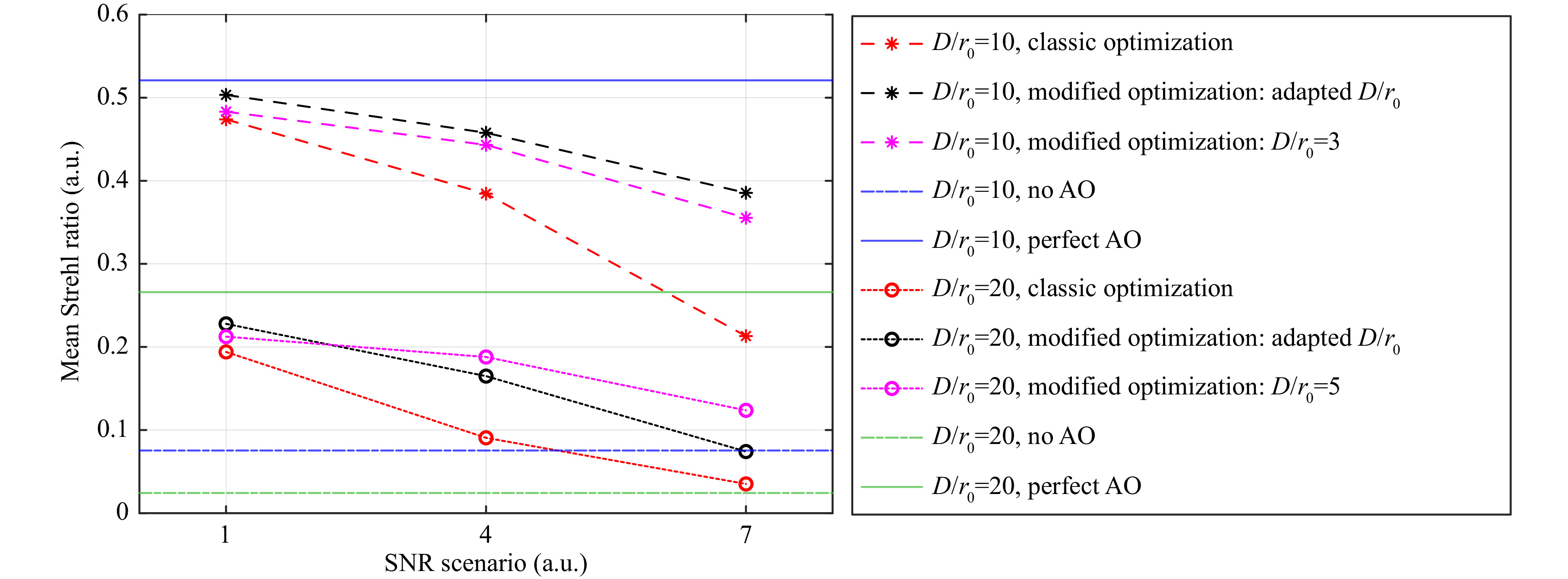

Fig. 11  Mean Strehl ratio for closed-loop AO with Karhunen-Lòeve-based HWFS, AO bandwidth of 1 kHz and AO gain of 0.3 when measuring and correcting 42 modes, shown for different SNR scenarios.

Although the modified optimization method is ideal for HWFS in closed-loop operation, it is obviously not ideal when closing the loop. Fig. 12 shows the instantaneous Strehl ratios over time for AO systems correcting 45 Zernike modes with a gain of 0.5 and a bandwidth of 2 kHz. The turbulence strength is $ {D \mathord{\left/ {\vphantom {D {{r_0}}}} \right. } {{r_0}}} = 10 $. The black curve represents AO with an HWFS that is optimized for this initial turbulence strength. The Strehl ratio increases almost directly to the level of the mean Strehl ratio. The blue curve represents AO with an HWFS that is optimized for the effective $ {D \mathord{\left/ {\vphantom {D {{r_0}}}} \right. } {{r_0}}} $. The measurement accuracy is lower initially. Hence, it takes more iteration steps and time to increase the Strehl ratio and reach the plateau. After this longer start-up phase, however, the Strehl ratio is higher. For very challenging scenarios with low signal and SNR and high $ {D \mathord{\left/ {\vphantom {D {{r_0}}}} \right. } {{r_0}}} $, the system that is optimized for the effective $ {D \mathord{\left/ {\vphantom {D {{r_0}}}} \right. } {{r_0}}} $ might not be able to close the loop at all. To avoid this in these special situations or to minimize the time to reach the maximum Strehl ratio, sensor design can be adjusted during operation: When starting AO, the optimal parameters for the initial $ {D \mathord{\left/ {\vphantom {D {{r_0}}}} \right. } {{r_0}}} $ are used and after closing the loop the sensor design is switched to the optimal parameters for the effective $ {D \mathord{\left/ {\vphantom {D {{r_0}}}} \right. } {{r_0}}} $. The dashed magenta curve in Fig. 12 shows the Strehl ratios when adjusting the parameters after 5 ms (marked by vertical dotted grey line). The Strehl ratio is raised rapidly and further increased to the higher level. The ability to adjust the sensor design during operation improves the stability of the AO system.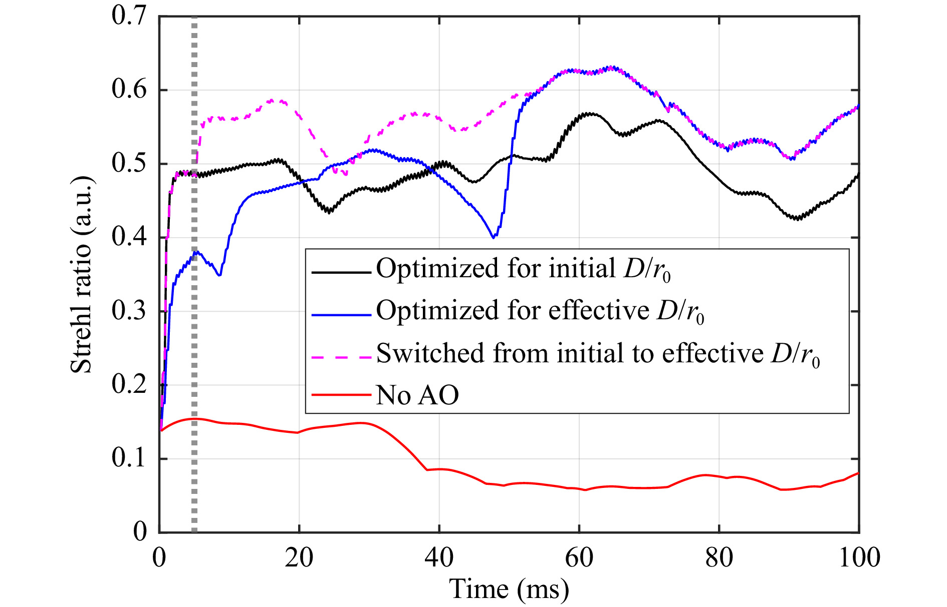

Fig. 12  Strehl ratio over time for closed-loop AO with Zernike-based HWFS, AO bandwidth of 2 kHz and AO gain of 0.5, when measuring and correcting 45 modes. The vertical dotted grey line marks the time when the sensor design is switched from optimized for initial to effective D/r₀ (dashed magenta curve).

Measurement accuracy, especially in noisy scenarios, can be increased by averaging over multiple successively performed measurements or by increasing the exposure time to improve the SNR. It has to be noted though that the increased measurement accuracy is accompanied by a reduction in the possible AO bandwidth. However, this problem can be avoided by designing the HWFS to carry out multiple measurements at the same time rather than one after another. When using an area detector for spot detection, multiple different HWFSs can be implemented without changing the number of spots or the biases for the modes. The spots are detected with different digital ROIs, i.e., for each HWFS the spot intensity is summed over a different number of detector pixels. The detector has to be read-out only once. Afterwards the sensor output can be calculated for several sensors with different digital ROIs and accordingly different calibration factors (Eq. 11). The total number of signal photons and the SNR differ for all measurements so that averaging over all measurements can reduce the influence of noise. The J-map, obtained during the optimization process, can be used to find the best combination of a number r ROIs with the same bias. For each row of the J-map the r smallest values are summed and the row with the smallest sum provides the bias (see Fig. 7b). With the corresponding calibration factors gained from the c-map, the r HWFSs can be used nearly simultaneously.

Fig. 13 shows results of closed-loop AO with a Karhunen-Loève HWFS using 1 (red), 2 (black) and 4 (magenta) digital ROIs. The mean Strehl ratio of the closed-loop operation is given for the 9 SNR scenarios (see Table 1). The AO gain is 0.3, the bandwidth 1 kHz. Results are presented for $ {D \mathord{\left/ {\vphantom {D {{r_0}}}} \right. } {{r_0}}} = 10 $ (dashed lines) and $ {D \mathord{\left/ {\vphantom {D {{r_0}}}} \right. } {{r_0}}} = 20 $ (dotted lines). Multiple-ROI measurements always lead to a higher Strehl ratio. The improvement of the AO performance is significant. For SNR scenario 9, the Strehl ratio is increased by a factor of 1.7 for both turbulence strengths when using only two different ROIs. Even for scenario 1 without noise, the AO performance benefits noticeably when using four ROIs.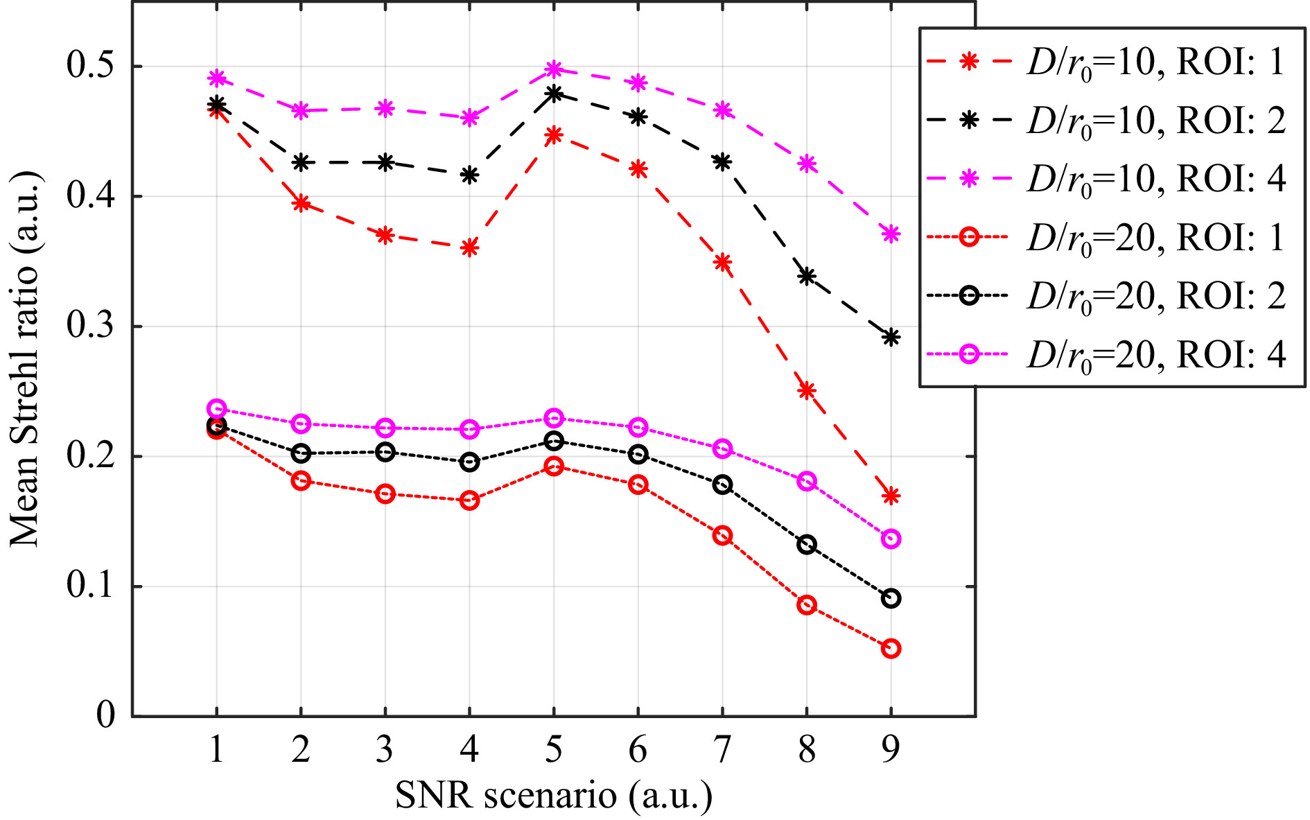

Fig. 13  Mean Strehl ratio for closed-loop AO with optimized Karhunen-Lòeve-based HWFS, AO bandwidth of 1 kHz and AO gain of 0.3 when measuring and correcting 42 modes, shown for different SNR scenarios. Dashed lines represent measurements at D/r₀=10 and dotted lines at D/r₀=20. The colors correspond to different number (1, 2 or 4) of used digital ROI.

The simulations show that a closed-loop AO system based on a HWFS is capable of correcting atmospheric turbulence. This is true even when bias and ROI are chosen based on common sense instead of optimization results. However, when using the optimization method that is intended for open-loop operation, the improvement of the Strehl ratio can be increased significantly. As expected, the optimized parameters are a good choice, but not necessarily the best choice for the changing conditions of closed-loop operation, especially for demanding SNR scenarios. Optimizing for the effective turbulence strength, i.e. the residual phase variance after closing the AO loop, has been found to be very effective. However, closing the loop can be problematic if a high number of modes is corrected and the difference between initial turbulence strength and the expected effective turbulence strength is too big. As shown in the previous section, adaption of the parameters to the current conditions increases the stability visibly. Changing bias and ROI during operation is not feasible for all sensor implementations. The holograms multiplexed in a hologram plate are fixed and cannot be changed afterwards. When using an SLM as DOE, the displayed holograms can be exchanged easily during the operation. The number of modes and with this the number of signal photons per spot can be adjusted. If an area detector like a CCD camera is used, the ROI can be changed for each mode at any time. With this combination the HWFS design is extremely flexible and can be adjusted to the turbulence conditions. On the other hand, the measurement speed of such a HWFS is limited by the readout speed of the detector. If the high bandwidth of the sensor is required, a fast photodiode array is usually used for spot detection. In this case, the detector size can be adjusted by means of a variable aperture in front of the photodiodes. Of course, this would result in an increase in complexity of HWFS. Instead of adapting the sensor design from initial to effective turbulence strength, we can choose a design that matches both conditions. By overlaying the J-maps of both optimizations, we can find a combination of bias and ROI that provides satisfactory results for both cases. Comparing J-maps of increasing $ {D \mathord{\left/ {\vphantom {D {{r_0}}}} \right. } {{r_0}}} $, we see that the combinations with the best results overlap. It is therefore possible to find a good compromise that ensures good stability even for challenging scenarios.

In addition to the modified optimization, the use of multiple ROIs increases the performance of the system noticeable. Nevertheless, this approach is also limited to the use of an area detector. Implementations with photodiodes are conceivable but significantly less practical. Using multiple ROI is particularly effective for low SNR scenarios. However, in these scenarios it is beneficial to avoid the use of many pixels in order to keep the readout noise of the detector as low as possible. When using multiple ROI, pixel binning is only possible to a limited extent. Therefore, the gain from the additional apertures must be weighed against additional noise. The limitations of the detector, such as dynamic range, have to be considered as well when designing a real system. If the detector has enough light available so that noise is not critical, it is always useful to implement multiple ROI detection at almost no additional cost. Especially high-order modes profit from the increased measurement accuracy.

The modal holographic wavefront sensor enables high-speed measurement of aberration modes in parallel. After detecting raw intensities, post-processing is limited to a fast contrast calculation for each mode. However, the measurement of one mode is influenced by the presence of additional modes. Especially when dealing with atmospheric turbulence, where the number of modes is infinite, this crosstalk effect reduces the measurement accuracy of the sensor. To investigate the usability of the sensor as part of a closed-loop AO system, we simulated realistic atmospheric turbulence. Choosing the design parameters according to simple, common-sense guidelines enables a respectable correction of the wavefront distortions. When applying an optimizing procedure that is developed for open-loop operation, we achieve a significantly better correction. However, especially for challenging SNR scenarios, we identify the potential for improvement. We modified the optimization procedure to take the new, residual conditions, i.e., the effective turbulence strengths, after closing the loop into account. This leads to a significant increase in performance and makes the HWFS usable even under difficult conditions. By using multiple HWFSs with the same bias but different digital ROIs simultaneously, we achieve an additional improvement and reduce the influence of noise. In the next step we will verify these results experimentally. We will create the HWFS as multiplexed computer-generated hologram displayed on an SLM and implement it in a closed-loop AO system. To validate the efficiency of the sensor optimization, we will use an 800 m free-space path through the atmosphere and monitor the improvement of the Strehl ratio during closed-loop operation.

This work was sponsored by WTD 91 (Technical Center of Weapons and Ammunition) of the Federal Defence Forces of Germany – Bundeswehr in the project ABU-SLS and by the Office of Naval Research Global under award no. N62909-17-1-2037.