A symmetry concept and significance of fringe patterns as a direct diagnostic tool in artwork conservation

In optical and digital phase-shifting holographic interferometry, a highly coherent ΤΕΜ00 diverged laser beam illuminates a surface undergoing static or dynamic displacement. The rest and new positions of the displaced surface are recorded and archived, allowing double—or due to recent developments in PC-driven algorithms—multiple, continuous, or interval selective monitoring of surface reactions. Recording depends on the problem being explored and the related methodology, with the goal of revealing substantial information. PC-driven recording is related to monitoring procedures based directly on a large number of surface datasets in the form of interferograms, with interference patterns characterizing the specific displacement of the surface in space and time under specific operating parameters and naturally or artificially induced excitation.

The displacement of a surface from an initial rest position indicates the rearrangement of the points at new positions. In the structural diagnosis of artwork, in order for displacement to be harmless in terms of the object’s physicomechanical properties and reversible elasticity, the excitation force needs to be very small (i.e., induce very little displacement) yet sufficient enough to induce displacement between all particles in the body relative to their reference position at rest in order to furnish high spatial information content. Ethically, minimal displacement in resolvable conditions in terms of the recording system and identifiable information in terms of diagnostic potential are prerequisites for artwork investigation.

Regarding artwork monitored under vibration-free strict stability requirements, displacement (strain) is not caused by changes due to rigid body motions but only due to changes in a) surface morphology due to local defects and b) surface size due to whole body dimensional movements, for example, shrinkage/expansion. The resulting displacement on the negative or positive z-axis is recorded in the direction normal to the axis, forming interference fringe patterns representing deformation with scalar optical path units of lengths (μm).

Fringe patterns are visualized as combined reactions of 1. “partial ” or spatially limited displacements (“local ” defects) and 2. “whole” extended areas of the surface (“whole” body spatial displacements, for example, shrinkage/swelling), and if referring strictly to dimensional (normal) deformation, the other components are negligible. The areas indicated by local fringe patterns represent “limited ” or “extended locations/areas ” with common deformation characteristics within “whole-body” displacement, a partial to whole body combination of information to become knowledge which is capable to describe the reactions and condition of the materials or layered constructions composing the artwork.

In the above context, the methodology presented here exploits how each interference fringe pattern reveals a physical tool to assess unique dynamic conditions and an approach that entails exploring them as representative information for the direct diagnosis of artwork, independent of other actions such as interactive measurements, unwrapping phase processes, FT or engineering stress and strain analysis. The objective of the methodology is to provide recognition steps for achieving direct diagnosis and automation reasoning.

In general, interference fringes are formed as a result of processes involving critical physical phenomena concerning wave physics and field superposition realized under the strict boundary conditions of the relevant physical laws. These laws are mathematically described, providing fringe pattern analysis with a direct quantitative information source indicative of the magnitude of the effects that the phenomena involved can reveal. The method allows for a highly precise quantitative study of the investigated surface.

The concept of incorporating holographic interferometry geometry for artwork structural analysis is justified by its advantages, starting from the scale of measurement, which, due to the incorporation of lasers, is of the order of a few micrometers, allowing small loads to be intentionally applied to successfully provoke small displacements without endangering the precious surface. The wavelength of light is added as a highly sensitive measurement for studying locally expressed invisible defects.

Implementation of hologram interferometry in structural diagnosis is based on the inherent property of field superposition in creating hologram interferometry, which allows a light wave diffusely scattered by an object to be holographically recorded and reconstructed with precision such that it can be interferometrically compared with light scattered by the same object at another instance in time^1–6. Interferometric precision denotes the accuracy and non-destructivity of the measurement, which are both critical properties in cultural heritage (CH) conservation research. Indeed, holographic interferometry, which provides an interferometric comparison (a holographic interferogram) of two or more waves, at least one of which is holographically reconstructed, is a technique that introduced laser applications into the CH field. Furthermore, it has been the basis of and provides a standard reference for the comparative development of techniques based on the principles of optical coherent metrology^7-15.

With regard to CH research, holography was introduced to art conservation and restoration applications not long after the invention of the laser.

Although there was intense interest in the application of lasers to CH soon after the laser’s invention, especially for cleaning and spectroscopy, research on the structural diagnostic capabilities of the holographic interferometry method to detect hidden anomalies was not progressing at the same pace, and there were only a few laboratories researching challenging topics related to holography for structural diagnosis of artworks.

In general, in the art conservation field, conventional conservation practices for structural examination require either well-equipped heavy installation facilities or time consuming and limited resolution techniques, for example, the commonly used X-ray imaging and finger knocking, respectively. The most commonly employed method to deliver a structural condition evaluation report entails transportation of portable artwork to an X-ray facility for examination OR by stereomicroscope and manual inspection. Even though these approaches have long proven to be effective, it is certain that traditional practices in the restoration of CH treasures, monuments, and museum collections are limited, and professionals are increasingly demanding new tools and practices in response to the impact of the deteriorating environment and the highly increased cultural demand for artwork exhibitions. Demand for new methods that are faster than the existing time-consuming procedures, integrated and non-fragmented instrumentation, sensitivity, accuracy, resolution and repeatability are all factors driving a new era in conservation tools that will allow for the transfer of technology know-how from laser research into the field of art conservation.

CH research that uses holography originated from certain laboratories that introduced holography and holographic interferometry techniques mainly to structural diagnostic applications.

Beginning in the 70s and 80s, Profs. Franco Gori and Domenica Paoletti published literature related to optical holographic interferometry and sandwich holography for painting and artwork structural diagnosis and continued later with electronic speckle pattern interferometry (ESPI) experimentation. Affiliated with the University of Aquila in Italy, the professors were very productive at applying holographic interferometry to panel paintings for defect detection and developing techniques for phase control, such as sandwich holography in which a carrier frequency input modulates the formation of interference fringes in the interferometric reconstruction process by using single optical holograms in temporally different acquisitions. It could be said that after Prof. Asmus’ first attempt in Venice, Prof. Paoletti and colleagues were the first to realize the power of holographic interferometry non-destructive testing (HINDT) in CH structural diagnosis and recognize holographic interference fringes as a unique tool to trace invisible hidden defects at determined locations and possibly correlate these with the defect type present in the artwork^16-21.

In the 80s, Prof. Pierre Boone at Ghent University in Belgium extended the use of holography and HINDT from application to mechanical problems to the study of defective ceramic and museum objects with video holography²². In several works, Prof. Boone explored three-dimensional (3D) representation applications of holography involving pulse lasers for producing high-quality portrait and naturalistic transmission and reflection holograms. In these 3D representation applications, important contributions advanced progress one step further. The 3D display can be attributed to Prof. Yuri Denisyuk and colleagues of the Russian Academy of Science, for their revelation of the unique 3D display properties of single-beam holographic representation in replicating museum objects for transport exhibitions via Lippman holography, which produced a large number of unique, quality single-beam holograms of museum objects, facilitating the founding of a holography museum in Saint Petersburg^23-25. Prof. Markov has also shown special interest in the 3D properties of holography and has contributed significantly to the idea of holography display applications for museums, while Prof. Boone worked diligently in the field during the 90s^{26, 22}. In another approach involving potential color holography, Prof. Von Bally and colleagues from Carl von Ossietzky University of Oldenburg, H. Bjelkhagen, and other scientists and PhD students contributed to color holography, aspects of display, and technical holography applications in museum practice, with particular attention to the quality of the reconstructed image, holographic non-destructive methods, memory, and image synthesis^{27, 28}. Prof. Von of Bally University can be credited for cuneiforms in artwork documentation. Oldenburg made further advances in the holographic remote study of archaeological objects²⁹. In the same period, Profs. Klaus Hinsch and G. Gulker, along with their colleagues from Carl von Ossietzky Oldenburg University, studied the use of speckle interferometry for the weathering deterioration assessment of monuments, an application critical for immovable CH as well as for the transfer of know-how from structural engineering applications to CH^29-31.

Regarding the contribution of coherent metrology and digital image processing to structural diagnosis, in general, significant advancements can be attributed to Profs. Juptner and Wolfgang Osten as well as their colleagues at BIAS, who elaborated on coherent metrology, surface inspection, and digital holography. Prof. Osten at BIAS and Institute Technische Optic University of Stuttgart, a visionist and organizer of international FRINGE conferences where the most internationally recognized holography experts gathered, made a unique contribution that has shaped coherent metrology applications, holographic interferometry, shearography, fringe projection applications, and phase-shifting interferometry. The development of BIAS’s FRINGE PRO software is specially mentioned here, as well as the mathematical analysis presented by Dr. Ulrike Mieth from BIAS, which, under the supervision of Profs. Juptner and Osten, elaborated the mathematical formulation of holographically-generated fringe patterns^32-36.

During the 90s, collaboration between Prof. Osten of BIAS and the author of this paper initiated systematic research on system investigation for CH, especially with regard to correlating the theoretical and mathematical models of interference fringe pattern formation with experimental data findings from actual defective and non-defective samples simulating structural defects in artwork^37-39. The joint effort produced an artwork defect classification table listing fringe pattern appearance and morphological symptoms indicating the presence of identifiable hidden defects. Hence, detection and definition through the interpretation and validation of interference fringe patterns facilitated a thorough classification of structural symptoms indicating types of defects based on holographic interferometry fringe patterns⁴⁰.

The author’s personal research since the early 90s started at Holography Laboratories at the RCA in conjunction with the V&A conversation department and the optical laboratories of ICSTM. After the elaboration of advanced holography display techniques, research was focused on the development of double pulse and double to multiple exposure holographic interferometry sequential recording methodologies to monitor reactions and study the environmental effects of dimensional changes in artwork. This research continued at IESL/FORTH with the development of defect detection and identification protocols, multi-exposure comparative holographic interferometry, and digital holographic speckle pattern interferometry in a lightweight portable remote access system termed the Digital Holographic Speckle Pattern Interferometry or DHSPI that monitors the environmental impact and traces defect conditions in order to study defect types and classification, defect growth and deterioration mechanisms, physical aging and interventive laser processes, preventive deterioration methodologies in direct monitoring in climate chambers, the role of defects in equilibrium processes, software development, and hybrid DHSPI instrumentation. Special interest was focused on interference fringe patterns as a unique tool in direct structural diagnostics for complex formations as a result of complex artwork constructions. In this paper, accumulated experience with the use of fringe patterns for defect and material reaction interpretation and implementation in direct structural diagnosis is presented and explained to guide future developments in AI^41-62.

Complementary relevant research on exploring the properties of speckle and shear interferometry has increased over the years, especially in the last decade, at a number of different laboratories that have produced a wealth of experimental and computer-simulated investigations to benefit the development of the optical coherence field in CH applications^{49-51, 63-87}.

The aim of this article is to highlight the unique properties of fundamental fringe patterns as physical tools and demonstrate their significance in revealing the structural condition and mechanical reactions of artwork, possibly allowing for automated evaluation.

Despite the widely applied displacement analysis approach that entails the calculation of engineering strain along with unwrapping interferograms, in artwork application, the direct approach requires in short measuring the fringe number from the zero-order fringe to calculate the relative displacement through fringe density per area and using differences in the interferograms’ fringe density to extract the “whole field” vs. tracing and classifying “partial fields”, thereby indicating “local” defect positions and types. A study on wrapped interferograms followed this procedure.

Interference fringe patterns are expressions of optical path changes for each fringe pair equal to half the wavelength with primary spatial frequency z = 0, depending on the angle of observation and wavelength.

fy=sinθ/λ, in mμ and/or lines/mm

The fringes wrap the phase of the wavefront carrying the displacement at the recording point. Fringes are directly quantitative, and their density is a number expressing the total displacement of the examined area of the surface in numbers.

Visual interference fringe patterns are regarded as a “physical tool” to measure the structural integrity of an investigated surface. This concept is straightforward. The displacement patterns follow symmetry laws. Symmetrical patterns are easily recognizable. Any homogeneous and isotropic surface under a normal small force generates “whole body ” displacement recognized in interference by the “symmetric ” intensity distribution. These are the symmetry architectures that can be used to define symmetry vs. the symmetry deviations of non-homogeneous and isotropic bodies, as is the case for any artwork that generates symmetric deviations closely related to specific archetypes. Local disruptions breaking the symmetry in the “whole body” symmetric intensity distribution indicate a “partial” loss of surface continuity generated by locally defined discontinuities, resulting in visible in fringe patterns local asymmetries. These locally defined asymmetries are also close to an easily recognizable symmetry archetype. Each indicates a specific type of discontinuity.

Thus, fringe patterns can be considered partial or whole body intensity distributions characterized by spatially limited defined symmetry and spatially extended defined symmetry, respectively. In an interferogram, the denser the localized fringe pattern formation, the larger the areas of spatially limited defined symmetry. These indicate the distinct subsurface and bulk characteristics that interrupt the spatially extended but defined symmetry indicating whole body displacement.

These local interruptions represent invisible defects hidden under the examined surface that are interferometrically traced and revealed due to their impact on the examined surface. Expert conservators familiar with the artwork’s construction and materials are usually needed to identify their cause, and once the local anomalies due to hidden defects are traced, the conservator studies and evaluates the artwork’s condition. To inform the conservator about the artwork’s structural condition, a defect map is generated based on the fringe pattern distribution covering the full surface, and the map initially serves as an on-site visual qualitative evaluation. The defect map could be sufficient to evaluate the conservation conditions and restoration needs through visualization of the corresponding defective surface areas. When distinct fringe patterns are visualised, as shown in Fig. 1, where it is seen that the whole field distribution, here of concentric fringes, is interrupted by locally distinct fringe patterns (features that interrupt the whole body fringes locally), this visual performance allows tracing of the defective areas while facilitates on-site evaluation of the risk posed to the precious surface.

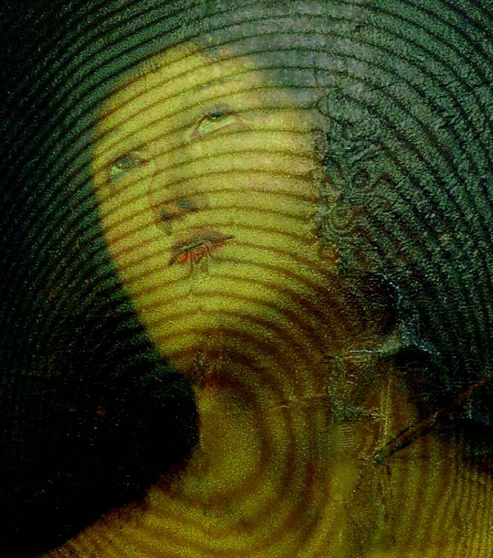
Fig. 1  Examination of a painting for structural diagnosis evaluation, where defect detection is clearly visualized in the surface abnormal distribution of fringe patterns. (Painting attributed to Rafael, in cooperation with the National Gallery of Athens).

According to the laws of interference physics, if there is measurable displacement within the scale of the measuring device, interference fringes are always formed, and the task is to record them. If locally distinct fringe patterns are not formed, then there is always a visible whole body fringe pattern covering the surface representing the reaction of the total surface area as a whole. The whole body fringe pattern signifies and measures the surface’s condition, its cohesion properties, and the overall integrity of the structure to a specific load.

Here, clarification of terms is essential to avoid confusion in the rest of the text. A “whole body” fringe pattern differs from a “rigid body” fringe pattern because of intentionally provoked displacement. The whole body fringe pattern is formed due to the surface’s overall reaction to deformation, whereas the rigid body fringe pattern is formed as a result of background noise affecting the x-y system’s stability, represented by linear distribution of the fringe pattern. The rigid body is linearly symmetric but distinguishable, as it clearly differs from the symmetry characterizing the formation of the whole body fringe pattern. Rigid-body fringes with stable equidistant fringes represent noise frequency. Experimentally, rigid-body fringes should be avoided by securing stability of recording system; however, there are applications where they can be useful as control for stability tests, for example, in paper interferometry where fringes on paper are expected to form within ns exposures using laser pulses the stability prerequisites tend to be underestimated since in such short exposures the rigid body fringes are rarely formed, unless recording system is fully unstable.

It is thus evident that holographic interferometry fringes are a reliable witness offering evidence of a successful interferometric experiment, as they demonstrate the efficiency of various excitation sources in terms of either naturally or artificially induced displacement. If excitation is capable of interacting with the investigated structure’s hidden defects, fringes are revealed on the surface, while the same fringes simultaneously provide information about the overall condition of the structure and about the setup interferometric efficiency. As shown in Table 1, the fringes are assessed:

It has been discussed how fringe patterns are assigned as 1.whole-body and 2. defects from the fringe distribution caused by displacement. In the presented diagnostic approach, the focus is on the direct diagnosis offered by secondary interference fringe patterns. The significance and manipulation of fringe patterns for direct structural diagnosis is based in understanding fringe pattern morphology and its use as a physical tool. Hence, the fundamental aim is to understand the fringe patterns as a picture or an image that, through special characteristics, provides information relevant to the structural diagnosis of artwork such that any conservator can directly proceed with diagnostic evaluation. Operation Diagram 1 shows visible fringe patterns for art diagnosis. These are termed secondary fringe patterns and are the fringes formed by at least two exposures and seen covering the surface. All the fringes, whole or partial body, which are extended all over the surface or limited to small areas, are secondaryinterference fringes that upon formation are visible to the naked eye.

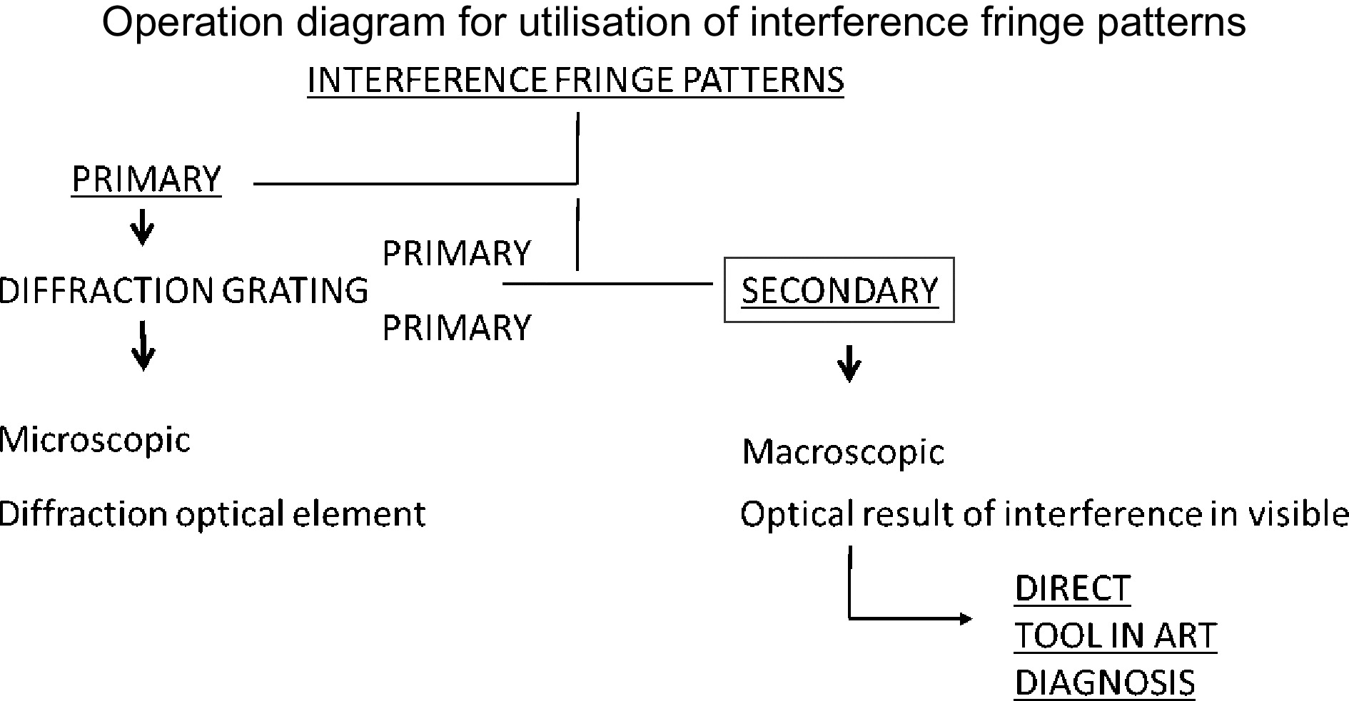
Fig. 0 

The method is very versatile and applicable to many different types of artwork with completely different characteristics. It can therefore become a universal tool in conservation, which means that understanding it as a direct physical tool is important. Interference fringe patterns’ unique properties and advantages as a non-destructive direct source of information suited for diverse applications and a variety of objects for which they function as a direct visual qualitative examination tool and a direct quantitative assessment tool are all inherently instituted in the interference phenomenon. Interested readers should refer to mathematical and experimental presentations of the classification table of fringe patterns for common defect types and an explanation of its validation in artwork^{36, 37, 41}.

Artwork and decorative art usually refer to complex constructions of multilayered superpositions. Each layer represents a different material or mixture of materials, potentially both organic and inorganic and commonly with different compositions and thicknesses. The schematic is shown in Fig. 2.

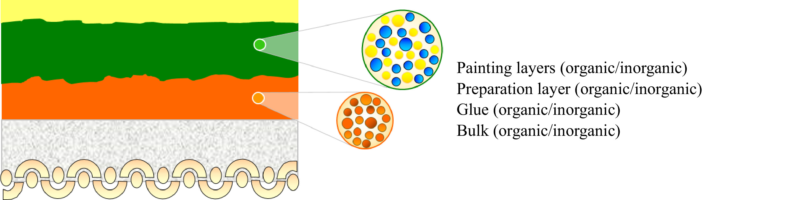
Fig. 2  Indicative cross-section schematic of a painting-like artwork.

When such a construction, considered to be inhomogeneous and anisotropic, and due to heterogeneity, lacking a representative volume element (RVE), is forced to move slightly by a few micrometers from its initial position predominantly in the +z or −z direction, that is, when it is forced to shrink or swell due to an artificial thermal increase or microclimate variation in humidity or temperature, the different elements forming separate density matrices move with different displacement amplitudes.

In our methodology, we are interested in the artwork’s exhibited displacement amplitude as a whole body and not each constituent layer’s ideal theoretical displacement amplitude. It is important that this is crystal clear, since the challenge in the art conservation field is to satisfy longstanding needs by adapting or creating engineering methods and practices for real, everyday CH applications.

The above description of artwork refers to flawless artwork, that is, artwork without defects, providing an idealized approach regarding materials and an even more idealized one with respect to the construction of artwork, which, by definition, suffers extensive flaws and defects. The fringe pattern approach, which is presented next, was used for defect detection via interferometry.

Artwork is composed of heterogeneous material opposed to the engineering of composite materials not typical to its mixture, as can be seen in the insert in Fig. 2, and since each artwork is a unique piece made of a pallet of ingredients, there is an insufficient number of common properties to support methodologies that embrace and evaluate the artwork as whole, unless one chooses to either destroy the artwork in order to study each layer separately (although this does not represent the artwork in its actual multilayered condition) or study samples and computer simulations^88-91.

In contrast, the holographic interference direct diagnosis approach investigates the artwork as a complete object. The fringe density (Δd/interferogram or area) allows us to obtain relative surface values of displacement that account for macroscopically uniform characteristics with respect to the applied boundary conditions of spatial heterogeneity and the RVE without destructive interaction with the constituent layers and materials^92-95. The fringe density/interferogram per area is calculated based on fringe number measurements using the concept of the zero-order fringe. The zero-order fringe is self-evident in interferograms because it is the RVE of the continuum of the material without any movement, so that in vibration isolation conditions or using relatively stable areas under in situ conditions with large or immovable artwork, the zero-order fringe provides a means to evaluate deformation within the mechanical description of the behavior of solid objects. This definition of motionless points as the RVE of zero-order fringes is related to art materials, as they are assumed to be a continuous mass, despite the fact that their matter consists of mixtures of discrete particles. The artwork is considered to be a continuum solid object allowing full-field measurements of small scale to be assigned to length scales far exceeding the interatomic distances, which, in turn, allows the study of physical phenomena such as the displacement reaction of macroscopic objects where displacement at different length scales cannot affect each other. This approach is theoretically steady because it is based on the interference field’s statistical ability to interfere with close and distant neighbor waves, producing a statistical effect representing surface displacement in the form of a fringe pattern.

In HINDT, the examined surface is considered to be a continuum surface acting as a diffuser when illuminated by an expanded coherent laser beam. The twice diffusively reflected light before and after a homogeneous force is applied interferes with a twin unmodulated reference. The optical path of the laser beam changes according to the whole body (excluding rigid body) displacement of the artwork’s surface in which each point of the surface is considered as a collection of points reflecting photons obeying coherent wave propagation, diffraction, and interference principles. The reflected photons statistically interfere with neighboring photons involved in the same path and change to produce displacement of the same phase change value, which gives rise to interference fringes extended in surface for as far as the phase value remains same. See an example of the principle of fringe superposition from interferogram reconstruction in Fig. 3a for a primary pattern (diffraction grating hologram) and 3b for secondary fringe patterns (interferogram).

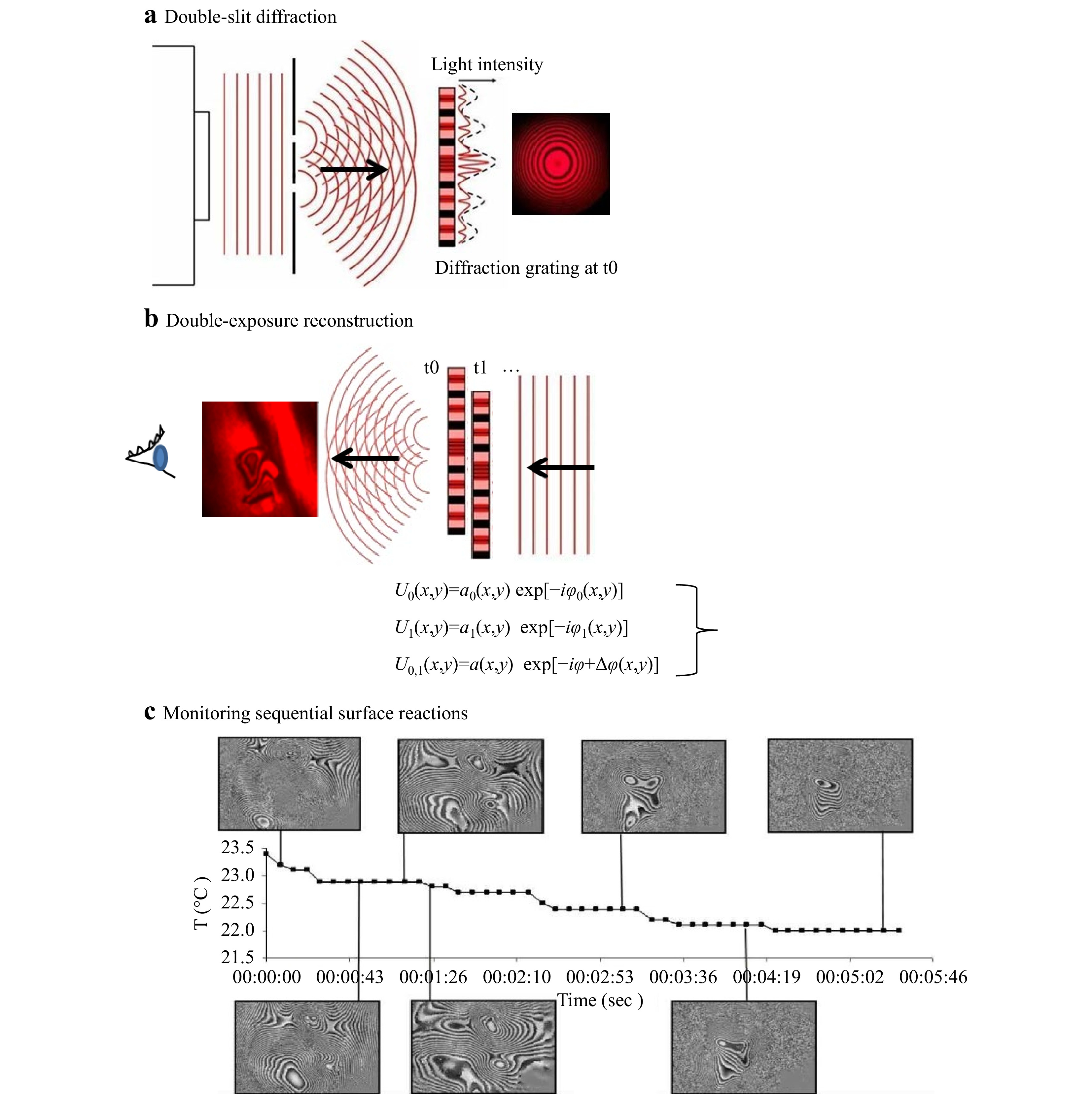
Fig. 3  Schematic representation of the developed real-time monitoring methodology of full field surface sequential displacement: a generation of a double-slit diffraction grating, b generation of interference between two diffraction gratings, and c monitoring dynamic displacements through the sequential capturing of interference fringes.

In Fig. 3a, a coherent plane wave field is deflected by a double-slit screen to emanate two mutually coherent spherical waves that spontaneously interfere, generating a primary modulated light intensity pattern forming a diffraction grating that is captured by a photosensitive screen at distance z. This formation gives rise to a fringe pattern (primary), and if illuminated, represents the interference field between the interfering waves. The secondary interference pattern that gives rise to visible holographic interferometry fringes reveals whole body displacement and partial fields; thus, potential defects are the superposition of two fields, where one of which has been provoked by a slight displacement force (not shown in this schematic). The change in dynamic requires continuous frame capturing and foresees a series of images from secondary patterns captured in sequential time events during relaxation of applied force or during continuous displacement toward reaching equilibrium with the environment, as shown in example Fig. 3c from a cooling down monitoring.

This is the sequential capturing utilized in the developed monitoring methodology, where hundreds of interferograms of each area as time windows of the area’s reactions are recorded and processed. The first wavefront U₀ represents the wave at time t = 0, where φ₀ represents the phase modulation from the surface of the object, while the interference between the consequent wavefronts is represented by the phase difference Δφ. In the first wave, the wavefront’s phase change is due only to the surface characteristics, whereas when the initial wavefront interferes with the wavefronts generated from the same surface after displacement, the phase change is formed according to the path differences that occur temporally in the surface wavefront.

As the surface wavefront changes over time, the visible secondarily formed interference fringes change the density following the change occurring on the surface of the object Δd = d₂−d₁. If, as in the case of thermal load, the object’s surface has undergone an initial transient impact, reaching its maximum displacement at the start time followed by lower displacement positions during relaxation, the same profile would be expected from the exhibited interference fringe density. The fringe density is shown to be the highest at the beginning of the measurement, with increasingly lower values until full surface relaxation is exhibited. The end of the process is indicated by a “no-fringe” surface, which signifies the end of the motion, ending the measurement. The displacement curve resulting from this process produces a fringe measurement, which follows the Newton law of cooling. Fig. 4 is the known graph of the Newton law of cooling, where the slope of the curve characterizes the rate of the cooling phenomenon dT/dt that takes place on the surface after thermal excitation. In the thermally-induced diagnostic methodology, velocity v(t)= Δx/Δt→ dx/dt dominates the fringe density in sequential interferograms and reveals acceleration of the surface and changing conditions toward equilibrium.

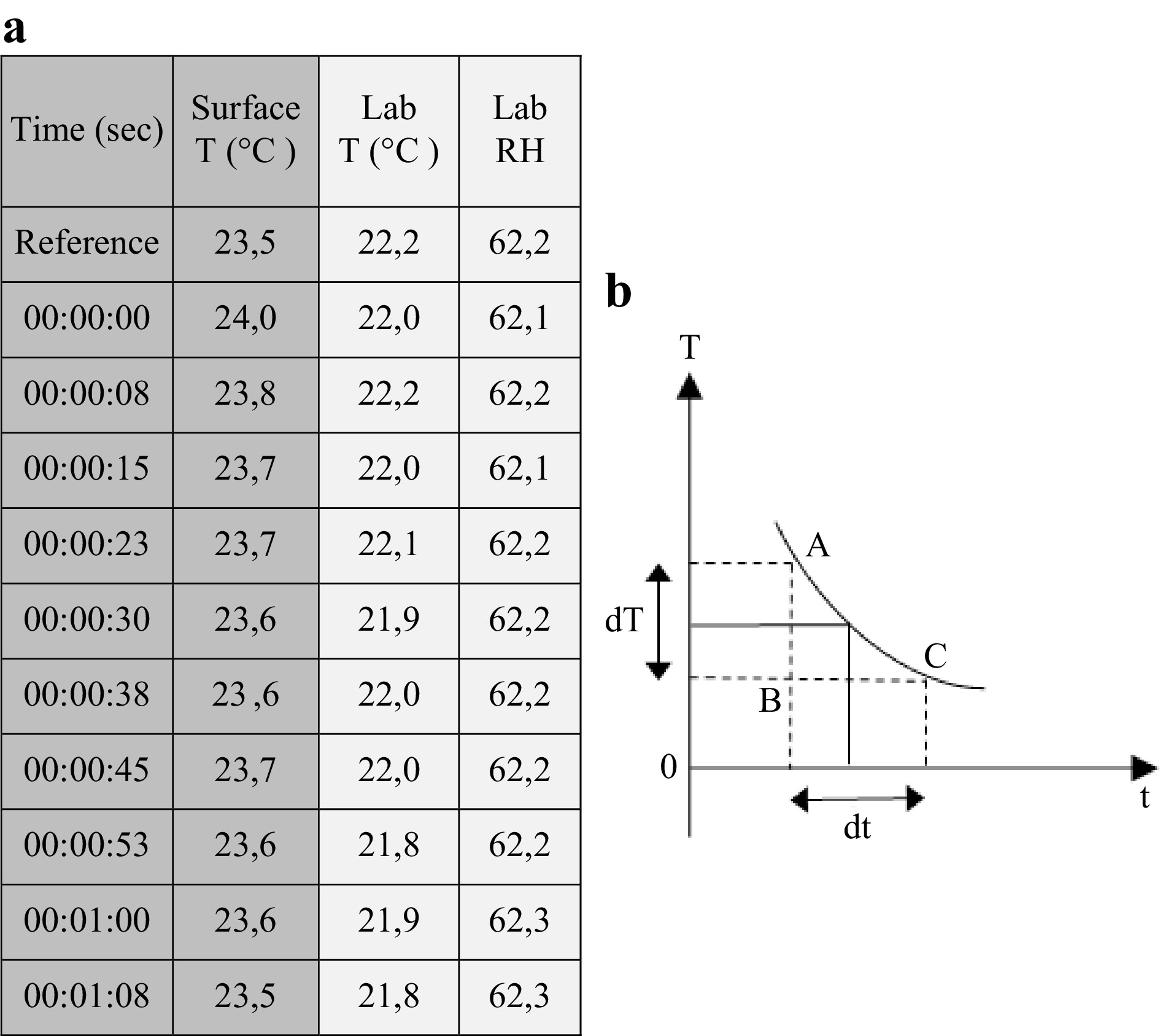
Fig. 4  Characteristic real experimental value table and theoretical mean curve slop during cooling.

Fig. 4 provides an example of the laboratory experiments. The relevant thermal load values of the time and temperature of the surface are shown in the table in Fig. 4 in the first two columns, while the lab’s relative humidity and temperature are shown for the control. If the thermal load is applied as an excitation force, the methodology for the measurement procedure starts with a ΔΤ = 0.5 °C, and in this example, it takes 68 s to return the surface to the initial value, with the mean acceleration of surface-temperature decay providing the rate of change of velocity

affecting fringe formation, so that it takes 8 s to 15 s for a 0.1°C change. In addition, as shown in the table, the very characteristic initial fast heat diffusion of surface loss in the first 8 s at 0.2 °C justifies the higher fringe density appearing in the first interferogram(s). These values, although dependent a) on the material and its condition as well as b) the parameterization of induced heat, specifically i) the type of induced heat, ii) the distance from the surface, and iii) the angle of the heat loader, represent a characteristic surface reaction after thermal loading. This method is implemented to generate the required fringe density for the defect trace, which, in turn, characterizes a) an artwork’s sensitivity reaction to the applied thermal load and b) the ability of thermal excitation to trace hidden defects.

The excitation duration measured in seconds is experimentally more suitable than the temperature difference (ΔΤ) and is used in unknown cases not tested before since the ΔΤ is not a priori known for a variety of artwork surfaces and mixed materials. To reveal the most possible information about defects and structural integrity, the excitation methodology requires extending the excitation duration that is applied step-wise from the minimum to the maximum in the interest of the artwork’s safety. Fringe density is again the criterion that will decide when the excitation increase will stop; the criterion is that the interferogram reaches irresolvable fringe density values, signifying unnecessary load excess. An example is shown in Fig. 5a−d, where a sample of a Byzantine icon is subjected to thermal excitation to perform a structural diagnostic procedure for defect detection, and the fringe density is increased at each step. In Fig. 5, only 5b is suitable for fringe counting, either manually or using automated software, because c and d have a higher irresolvable fringe density.

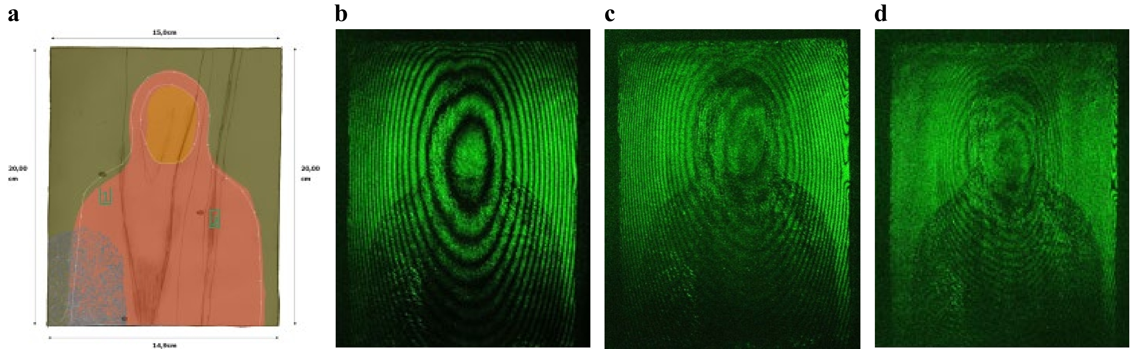
Fig. 5  Exemplary fringe density change as reaction to different parameters for applied surface acceleration using homogenised thermal load in a the byzantine icon sample; b 1 s, c 2 s, and c 5 s of applied excitation duration.

The fringe contrast in Fig. 5b−d seems to decrease because the fringe density increases, making the fringes irresolvable with regard to being measured, photographed and studied. The interferograms show the effect of fringe density as a product of optical path changes, such as increasing displacement provocation.

Procedure: The fringe density is measured depending on the complexity of the interferogram on one to three axes on the raw interferogram either by a) visually counting the fringes from zero-order or b) using an automated software to measure after unwrapping the number of fringes from the fringe skeleton, with the operator interactively setting the zero-order point from which measurement starts. Quantitative evaluation of interferogram fringe counting via either method is a prerequisite. To start measuring a) manually, after the zero-order point is established, it is essential to recognize the characteristic symmetry of the fringe patterns, which entails the controller directly ascertaining the fringe number and density measurements without duplicating the values. If the symmetry of the displacement (whole field) is not recognized, the error of doubly adding fringes is possible. In cases of extreme aging and complicated fringe patterns, which are common in artwork diagnostic examinations, requiring a deep understanding of fringe pattern formation, the rule of whole field symmetry may collapse, and symmetry recognition should be applied locally on each pattern, indicating an isolated defect. When b) measuring using software, if unwrapping is possible, a priori knowledge is required to set the zero-order point, and fringe counting is performed automatically, but in complex cases involving aging, unwrapping collapses, and symmetry recognition in the whole or partial field is necessary to evaluate the interferograms.

The fringe density exhibited in the visible interferogram is the secondary spatial frequency of the two interferograms that witnesses the body’s reaction to the induced load, here thermal load. Thermal load is applied in the present diagnostic procedure, to generate controlled surface displacement for the structural diagnostic purposes. As the surface’s temperature increase is internally absorbed, it influences heterogeneous construction by exerting different impacts on its constituent elements, which have diverse thermal coefficients. These, in turn, are differentially displaced, provoking diverse displacement impact on the monitored surface. Hence, if there are hidden defects in the subsurface, even when they are attributable to different/ materials, if affected by the load, they will exert a visible impact on the surface.

With the recording methodology of sequential monitoring applied throughout the thermal cooling of the artwork’s excited body, differential displacement is captured in time as it influences the body, starting from its surface, and diffuses into the depths of its construction. As time passes after excitation and while the body cools down, thermal excitation diffuses into the structure from the surface to the lowermost layer, visualizing the impact of the defects on different layers at different depths. The longer the duration for which a defect impact appears on the interferogram, the further it extends in terms of depth, revealing extended disintegration of the subsurface layers and bulk; conversely, the shorter the duration of its appearance, the less pervasive it is through the object’s volume, and the more restricted its influence to a certain depth is. The critical defect diagnostic parameters are when and for how long the defect appears. Hence, the defects’ sequential recording positions the defects in the depth of the construction and defect depth is indirectly evaluated.

Risk index: To gain preliminary information about each artwork, we perform zero-order fringe identification (defined as the part of the object with no displacement) either manually or via interactive software on one or more axes. In direct (manual) fringe number measurement, a different fringe density for each direction axis in the interferogram, either as a fringe number or as a product of wavelength Nλ/2 (N number of fringes in micrometers), is assigned, and the mean value is extracted. The mean value changes in the presence of a defect, allowing numerical differentiation of the defect and the whole body.

The whole body fringe density measurements, in a direct defect diagnosis investigation with homogenized transient thermal load over the surface, fit as expected in the theoretical graph, as shown in the graphical representation given in Fig. 4, based on experimental values. A theoretical graphical representation based on experimental values taken from a sample with a known defect was verified. The data were obtained from measurements taken both from the whole body fringe pattern and from partial localized defects. The result visualizes the differences between whole and partial field reactions due to existing defects, as presented in Table 2 as values and graphically in Fig. 6. The partial body representing the areas with defects clearly exhibits a higher number of fringes, producing an intense local fringe density either in excitation duration parameterization Fig. 6a and during the cooling down after excitation Fig. 6b.

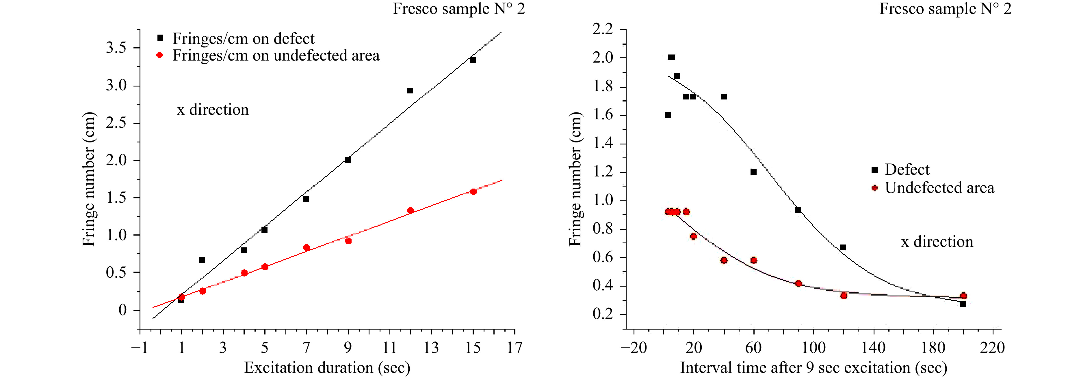
Fig. 6  Graphical representation of fringe density for partial vs. whole body differentiation.

Table 2 shows that excitation duration is a more controllable and repeatable parameter than ΔΤ. Fringe density changes can differentiate displacement along the same symmetry axis, distinguishing whole from partial body and indicating the defect area. In the particular example of defect detection based on fringe density, the detected defect is located 5 mm under the surface and has a strong impact on the surface in almost all experimental thermal ranges. The defect isolation and measuring procedure is possible for as many defects as are isolated in the whole field interference fringe distribution, resulting in a surface risk map with an itemised defect risk index, as shown in the example given in Fig. 7a, b (painting attributed to Rafael; cooperation with National Gallery of Athens).

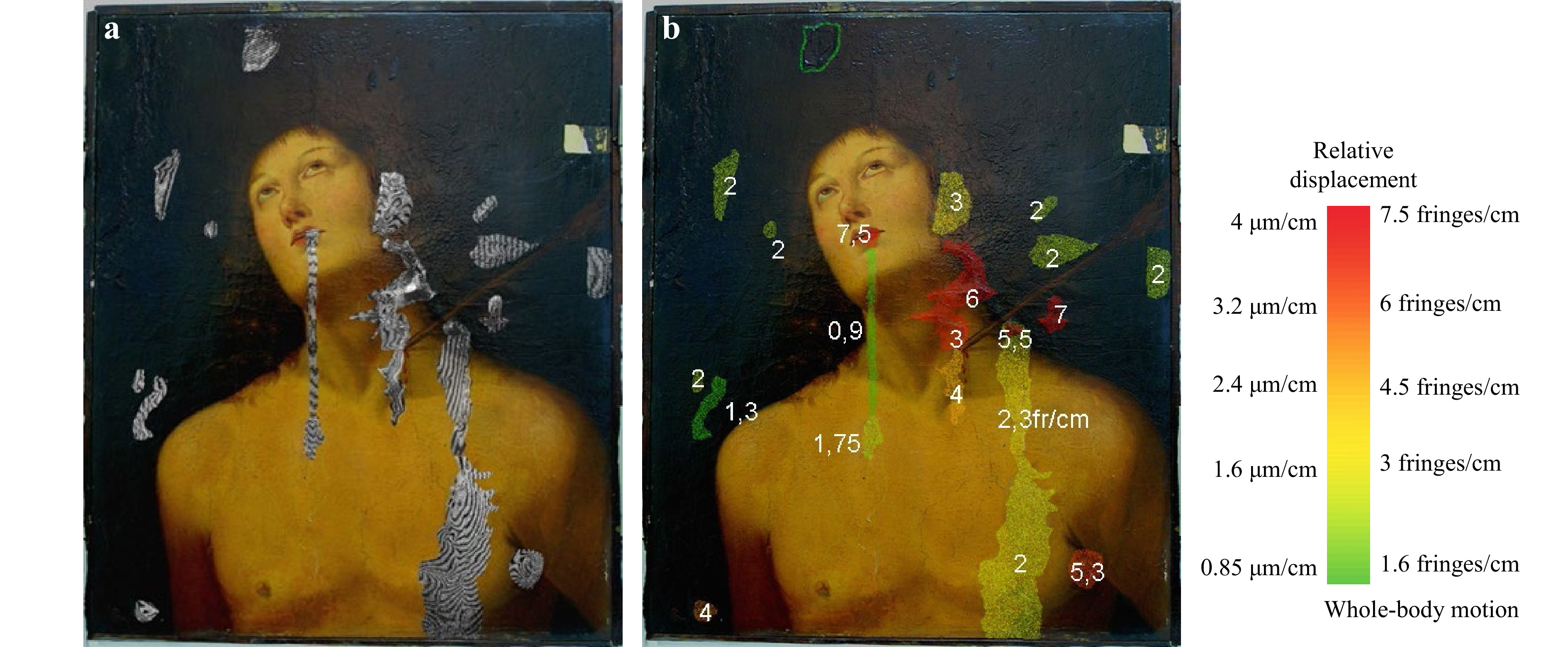
Fig. 7  Investigation for assessment of risk damage in painting surface. In a defect isolation and b defect risk index resulting from measurement of whole body vs. defect fringe density. (*NGA courtesy)

Fringe number measurement, either from zero-order fringes in lab vibration isolation conditions or relatively in situ, large surfaces and immovable conditions, that is, the defect isolation method, facilitates risk prioritization to serve as setting priorities in the restoration strategy. Following this map, a conservator can decide which defect exerts the most significant impact on the precious surface at the outset, considerably reducing restoration time. Fringe measurement can be performed in situ directly from the visible raw data after establishing the non-excited area (zero order fringe) and can be further post-processed in the lab using other software tools to study other defect characteristics. The fringe density, if needed, can be analyzed further by applying locally developed post-processing software routines, which provide additional information about the defect’s impact on the precious surface, detailed coordinates, shape, micromorphology, defect interconnection, etc. Thereafter, the itemized defect risk index can be generated and utilized as an early warning prioritization tool in everyday conservation practices, assisting conservators in their decision-making interventions.

In addition to the significant parameter of fringe density, that is, the method of realizing measurements of the displacement of the artwork’s surface based on fringe density, which has been shown to provide evidence of differential reactions within the surface, allowing for the location of intensity distribution abnormalities termed whole or rigid body vs local defects and assigning risk index of the impact on the surface, there is another important feature of interference termed fringe patterns that produce visual data of intensity distribution formation and provide significant evidence of local anomaly or the type of defect. In this process, symmetry deviation is the significant parameter.

Fringe patterns, especially dense fringe patterns, may appear to be random abstract formations, but they are not. Indeed, Dr. Ulrike Mieth (PhD Univ. Bremen – BIAS collaboration) has proven that they can be described through linear and non-linear partial differential equations, and she provided a thorough mathematical explanation of each of the most commonly appearing fringe patterns⁸⁸. Based on this study we later confirmed experimentally the mathematical and simulation approach, with greatest possible fidelity of the resulting correlation. All different approaches resulted in the same pattern classes that were used to define the type of defect with high accuracy^{35, 41}.

Fringe patterns are described as visual mathematical entities exhibiting symmetry, order, and limitation, the qualities of which are found in symmetry property exploration^88-101.

Some fringe patterns exhibit reflection symmetry, where two halves of the pattern are mirror-like or perfectly coinciding if folded, as shown in Fig. 8, which provides a recognizable characteristic example from a typically symmetrical shearography pattern representing the deformation gradient. It should be clarified here that the “mirror-symmetry” of shearography wrapped patterns due to self-reference is characterized by dual mirror-type symmetry, independent of the existence of defects.

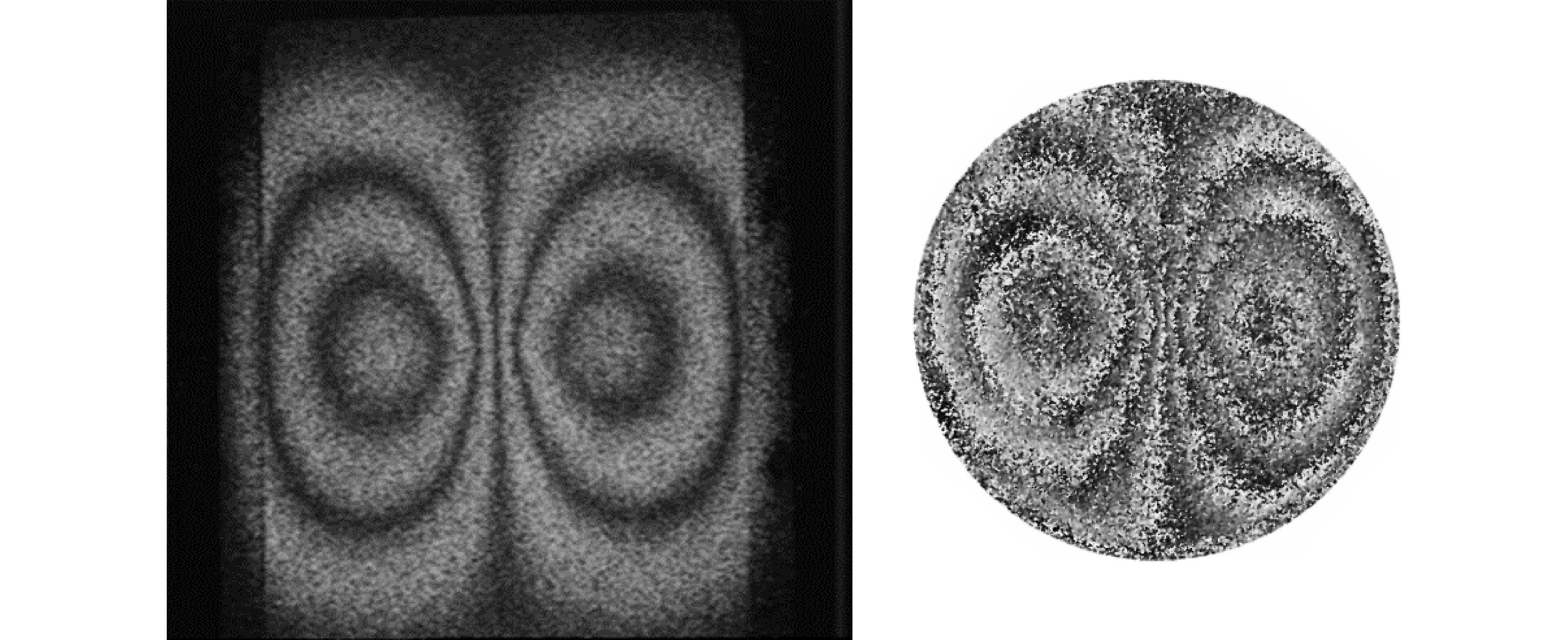
Fig. 8  Mirror symmetry exhibited from interfering two twin coherent beams, with one wavefront sheared with respect to the other, to assess deformation gradient from shearography pattern.

Scale symmetry is exhibited in fringe pattern formation without constrained object dimensions, which are observed to appear as the same, independent of scale, meaning that the same fringe pattern is exhibited whether from a tiny object made of any material or a larger object made of any material (material effect fringe pattern). The scale symmetry pattern is a remarkable effect, as it ignores the object’s dimensions and scale. Examples of this symmetry exist in interference fringe pattern formation during the investigation of artwork such as wall paintings, panel paintings, and sculptures; large and small objects exhibit the same symmetry under displacement^{35-37, 41}. One would think that fractal mathematical laws play a role in the generation of these fringe patterns.

Complex fringe patterns prompt fractal geometry, exhibiting a form of scale symmetry and exact or approximate self-similarity; that is, the entire fringe pattern has the same shape as one or many or all of the smaller parts constituting the fringe pattern, as shown in Fig. 9.

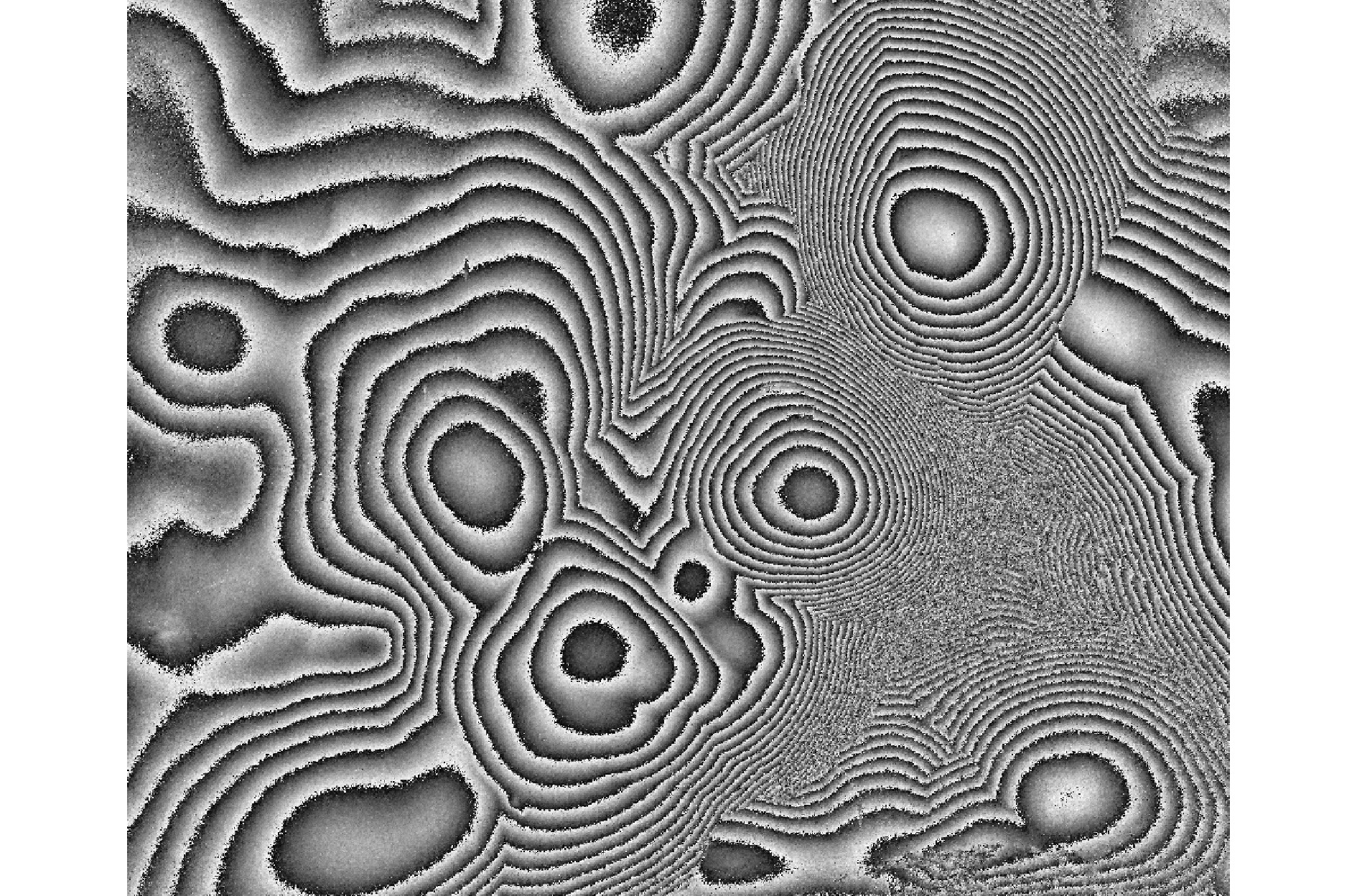
Fig. 9  Wrapped interferogram from a wall painting exhibiting multiple similar-symmetry circular-type fringe patterns of different fringe densities.

Smaller parts that are similar in shape to larger parts, regardless of dimensions and scale, which is common in mathematical fractal generation, are typically found in hologram interferometry fringe patterns. This symmetry is observed in complex deteriorated artwork where holographic interferometry patterns are produced during the displacement of aged artwork carrying multiple internal defects. These interferograms are the most complicated, exhibiting similar fringe patterns in multiple dimensions within the same but larger-scale fringe pattern; these are mostly exhibited in artwork-induced displacement for diagnostic purposes, as shown in Fig. 9. Disorganized matter generates similar displacement patterns, and the greater the degradation of materials, the more complex the fringe patterns that need to be unwrapped and evaluated. Hence, automation algorithms fail in such cases, and the whole to partial body and symmetry approach helps to locate and isolate the defective areas.

In Fig. 10a−c, characteristic cases of symmetrical whole body interference fringe pattern formation are shown for three different types of coherent interferometry techniques. Each interferometry technique generates an interference phenomenon that affects the formation of the fringe pattern; however, symmetry remains a common property in all techniques.

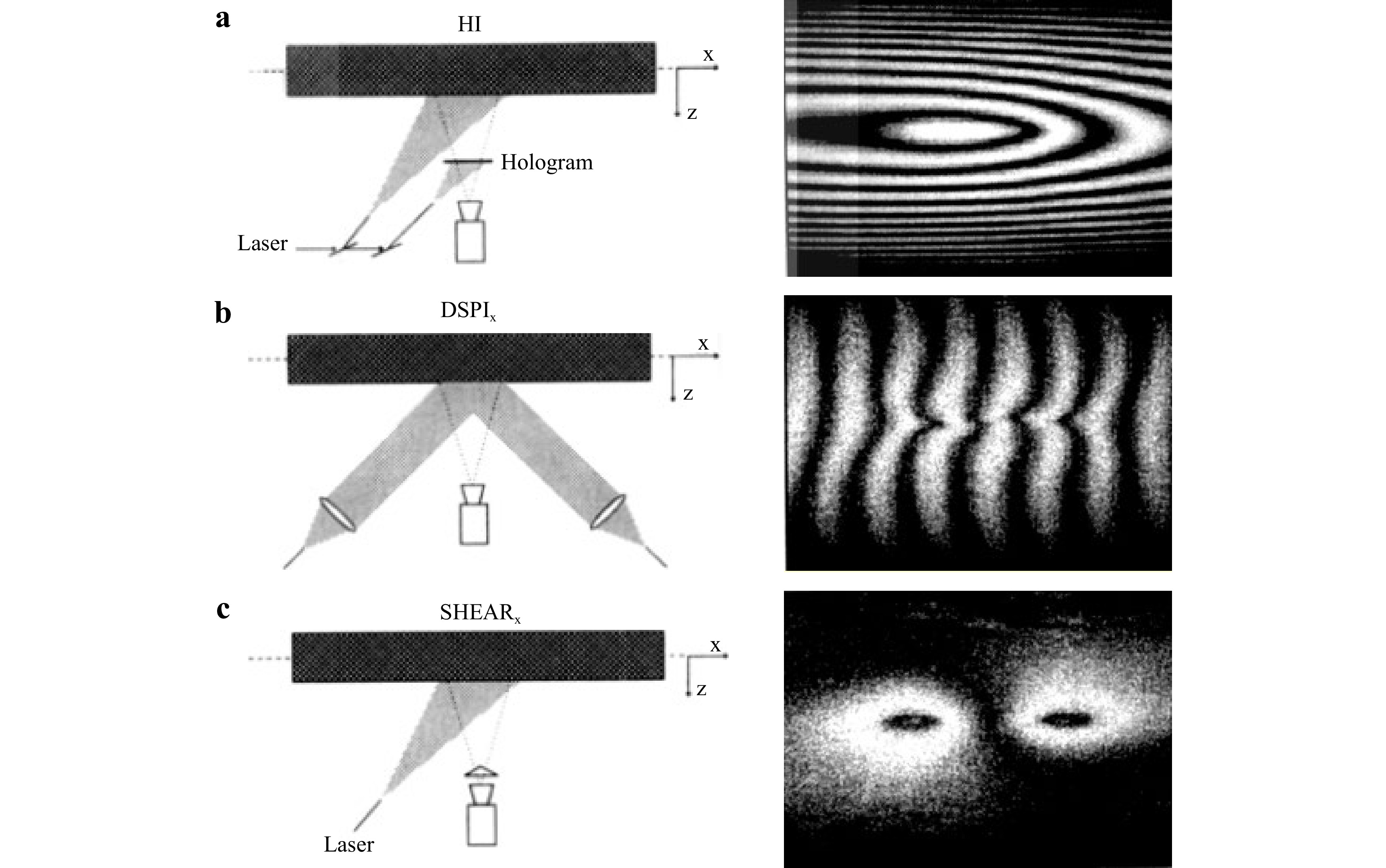
Fig. 10  Examples of the exhibited symmetry investigation of the same sample in a real-time holographic interferometry, b speckle interferometry, and c shearography.

Revealing the “whole from a part”, as in optical holography, describes an idealized symmetry property. If just a portion of a developed optical hologram is illuminated the whole of the recorded image is reconstructed. By changing the illumination direction, the whole image is reconstructed following the different viewing angle.

In natural objects, as in the impressive phenomenon of the structure of snowflakes, a symmetrical portion of the snowflake’s tip is repeated throughout the whole snowflake. This description reminds us of the unique feature of holography recording, where one viewer can see the entire recorded scene from just a small part of the optical hologram. This is the “interconnection” property of the primary fringes of holograms forming a diffraction grating from any random object if the object has been coherently illuminated and the recording medium receives the reflection from the surface. In an optical hologram, interconnection and reconstruction of information about the entire scene lead to visualization of one of the exotic properties of optical holography. This property can be demonstrated via a holographic film: if a hologram can be torn apart in small pieces, and each single piece, no matter how small, is illuminated with coherent light, each small piece can then be reconstructed to reveal the whole field, each from the viewpoint of the film’s light-receiving angle at the time of recording, with parallax limited by the angle of and information in the piece. It may be that the tiny piece of the hologram can be regarded as holding all the information about the whole, as with the tip of a snowflake.

It is suggested here that the holographic interconnection property be considered a type of paraxial symmetry with a conserved quantity, where “symmetry” is defined by the axis of propagation for angle of observation φ in the case of horizontal parallax and θ in the case of vertical parallax. In holograms, regarding symmetrical paraxial quality preservation in holographic paraxial viewing, the entire scene is conserved despite the change in the viewing angle, suggesting that perhaps even seemingly random and complex objects and scenes are folded symmetries, or, according to Noether’s theorem, “Any symmetry in nature has a corresponding conserved quantity”¹⁰².

The property of fractal organization defined as “self-similarity independent of scale, in all scales” is a highly extended property in hologram interferometry, in interference fringe patterns where self-similarity is observed as the same symmetry patterns formed interferometrically from different objects made of diverse materials with unrelated constructions and in different scales. Whether a tiny object or large scale object is investigated same variance of symmetry patterns arise making impossible to extract the scale of the object without prior knowledge.

Careful experimental or computer simulated investigation of various materials under homogeneous thermal load reveals that inorganic materials predominantly exhibit in-plane displacement with parallel isopach isoline fringe patterns, while organic materials predominantly exhibit out-of-plane fringe patterns in concentric circular interference fringe pattern arrangements.

Wood is a particularly interesting organic material because of wood cutting. The wood cut determines fringe pattern formation, regardless of the type of wood. The wood cut makes distinct fringe patterns that are distinguishable from other wood cuts. When different wood cuts are interferometrically tested, they exhibit characteristic fringe patterns that indicate the type of wood cut. However, characterizing wood material through the fringe pattern is more complicated, and a database generated with strict boundary measuring conditions is required.

Despite the physical interest that the exhibited symmetry holds for revealing order in complex systems or even providing clues to the deeper order of the universe, the idea of our methodology is to use the expected symmetry of whole field interference fringe patterns to trace, through asymmetries or local collapses of symmetry, the hidden impact of defects on the surface, independent of the pattern’s complex organization and use the fringe pattern’s appearance, regardless of how small or distorted it may be, to locate and identify, through fringe pattern classifications, the type of hidden defect. In this context, the most common computer simulated and experimentally derived fringe patterns have been investigated using known defect samples. Experimental results have delivered fringe patterns that have been shown to be fully correlated to load and defect.^{36, 38, 41}.

Given that symmetry is a way to order nature, and fringe patterns exhibit symmetry, they can help to order highly complex interference responses. In physical phenomena studied under symmetry theorems, when symmetry breaks, there is a cause, and the same can be expected in examined cases of hidden defects’ impact on an artwork’s surface because any localized impact on the surface breaks the whole body symmetry of the surface displacement.

For use with artwork specifically, direct structural evaluation, which is actually the practical aim of the development of the concepts and methodologies presented here, via the analogous geometric topology approach is implemented in order to exploit the idea of the “symmetry of whole body fringe patterns” and use it as the basis to distinguish “whole field displacement” from “partial field displacement” to identify localized irregularities. Using this approach, the interferometry fringe pattern of a displaced surface described geometrically falls within one of three possible geometries, as shown in Table 3.

The above classification fits the intensity distribution in the formation of fringe patterns and can be implemented safely for use in everyday evaluation to perform direct, fast structural diagnosis.

When a plane surface (d_x, d_y) undergoes a homogenized induced or natural displacement (d_z), as previously described, the recorded whole body secondary interference fringe patterns correspond to the description of possible geometry topology surfaces in Table 3. Nematic field topology geometry has been observed in high-complexity fringe patterns, as in aged and highly deteriorated primarily organic multilayered artwork^101-102. However, this case has not been classified here because it cannot be experimentally proven since this complexity cannot be repeated to create a classifiable example. Given that age or material cannot be considered representative of a sample, and a database does not exist, the case is not included in the experiments. The main difficulty in including the case is that a plethora of real samples or known defect samples are needed, and these are not easily found or constructed with precision. Thus, the nematic field was excluded from the classification.

It is clarified here that in most experimental cases, the displacement direction is known, and it can be determined via classic displacement vector analysis relating the motion direction to one-, two-, or three-dimensional surface displacement^10-13. The displacement vectors describing the surface displacement are mostly suited to engineering analysis for position determination. However, by applying the symmetry approach to the distinction of whole and partial fields for direct diagnosis and defect detection, the process becomes visual. In this approach, topology and continuous symmetry breaking in soft matter are more suitable and relevant mathematical theories that better satisfy the presented methodology^{101, 102}.

The delivered fringe patterns of surfaces exhibiting displacement, without exhibiting the impact of any internal defect, are covered by intensities that have a normalized distribution interchanging between the maxima and minima of the light intensities forming the fringes (recorded either analogically or digitally). This is shown in the identity function id(x) taken from the optical interferogram given in Fig. 11. Interferogram symmetry is evident, with minor deviations from symmetry, and can be idealized in surface geometry (Figure 11ciii, diii bottom). For interferometrically visualized surface displacement, as in the case depicted in Fig. 11ciii, if direction is important, vector analysis is needed because there are two possible negative and positive displacements of the geometric topology, as shown in Fig. 11dii, diii.

Fig. 11  Fringe pattern symmetry to surface topology: a surface geometry analogy of whole body displacement.

The other case for vector analysis if direction is important is on-line displacement, that is, x or y displacement, corresponding to flat surface geometry (Fig 11bi, ii−di). If a load is mechanically induced, it simplifies the evaluation because the direction is known. However, even with a 3D load, as in the case of thermally induced or environmental provocation of a natural impact, the displacement is deduced if the measurements of temperature (T) and relative humidity (RH) are taken during the experiment, and an association can be established, as shown in Fig. 12a−c. There, an increase or decrease in RH is monitored, and the surface geometry is deduced from concentric fringes that correspond to an increase in positive curvature, while a decrease is negative. Due to this additional information, the direction is known (+z increase: swelling, −z decrease: shrinking).

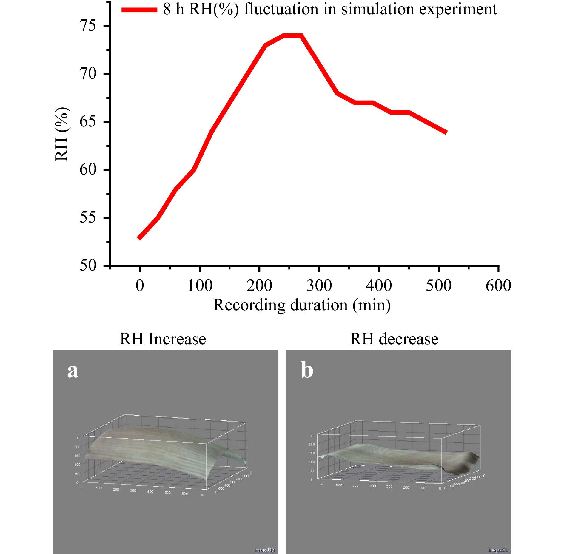
Fig. 12  Increase or decrease in RH is monitored, and the surface geometry is deducted from the fringe pattern.

Hence, one-to-one correspondence between points is used to determine the type of displacement by identifying the surface geometry, as shown in Fig. 11a−d. This fully applies to the linear in-plane displacements seen in Fig. 11bi, ii–ci, and ii–di, where the dominant whole body displacements are parallel fringes arranged in the x and y directions.

The correspondence between mirror points of symmetry in the concentric fringe pattern related to dimensional displacement generates a spherical or hyperbolic curvature in the fringe pattern, as shown in Fig. 11biii−ciii−diii. It is implied that this determines the type of displacement in the two cases given in Fig. 11diii, given the known dimensional load and monitoring of the values, which can correspond to fringe pattern formation.

The whole field fringe pattern is then used to extract partial fields to locate defects. If the data is too big for manual exploration, the developed software next dscribed and shown in Fig. 13 is used to automatically scan the wrapped raw data.

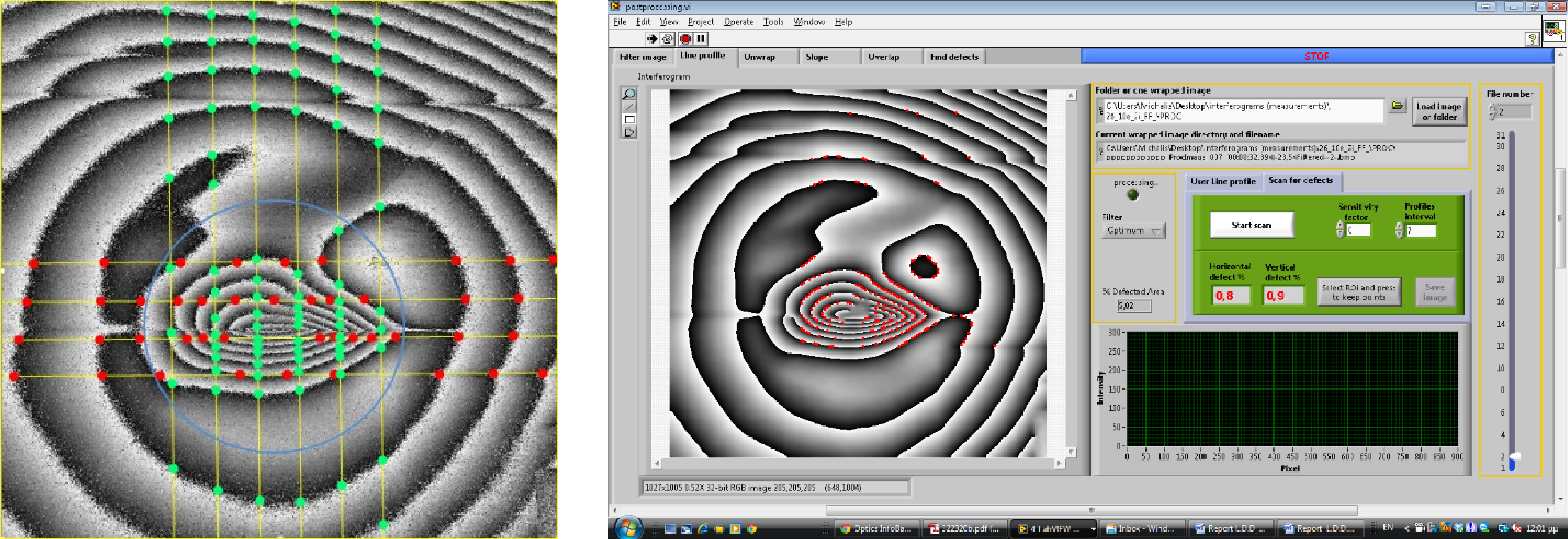
Fig. 13  Example of the developed automatic tool to extract defects from whole-body fringes.

For interferometry fringes to find a special place in art diagnosis, the automatic detection of defects is very relevant to any effort. In this context, an effort to a scanning algorithm developed to automatically locate defects is shown in Fig. 13a, used directly on a real example of a defective symmetric fringe pattern; the whole/partial field fringe density is directly evaluated, as explained and defect is extracted as shown in Fig. 13b, and extracted. The procedure is repeated for as many axes as required to minimize error. The procedure starts with a chosen axis such as x or y and the diagonal. Each chosen axis is then scanned as many times as required to deliver the data, as in the manual case shown in the last column of Table 2. Scanning can also be performed manually on interferograms that directly exhibit whole vs. partial body displacement, but using processing tools in post-processing software, interferograms can be uploaded automatically and evaluated in sequence.

A scanning example of a characteristic symmetry break due to defects is shown in Fig. 13a, b.

The determination of whole- vs. partial-body fringes and the quantification of effects due to load or defect are performed by assigning spatial fringe density, as shown in Table 2. The aim here is to use automatic evaluation and scanning to accurately localize the defect’s appearance. ω₀ is the overall induced frequency that generates the whole body, and ω_def is the deviation of the overall displacement visualizing the partial field. The step-wise process is described below.

The first step is to count the fringes of the interferogram with line profiles on both the x and y axes (Fig. 13). The step in each axis is user-defined and depends on the interferogram’s estimated fringe density/area in cm or mm. This is the method of extracting the sum of fringes in each line profile along the x and y axes and then calculating the average localization value ω₀. Here,

The next step is to compute the sum of each line profile exceeding (or not) ω_0x (for X scanning) and ω_0Y (for Y scanning); their sums are ωX⁺ and ωX⁻ (X axis) and ωY⁺ and ωY⁻ (Y axis). The equations describing the procedure are as follows.

For the X axis,

For the Y axis,

where ω_x,y are the edge coordinates along each line profile across X and Y scanning, respectively.

Once we have found the numerical values for ωΧ⁺, ωΧ^-, ωΥ⁺, and ωΧ^-, we are ready to calculate the basic equation that indicates the localized deformation deviation. The result of this equation is a number that shows whether the structure has a local deformation. This number must be greater than 1 in order to assume a defective image. We use the following equations:

The development follows the order shown in Table 4:

The values stored in programs’ memories are resynthesized at the end of the interferogram procedure to emphasize the deviation from the norm in a separate result file, as shown in the example given in Fig. 14.

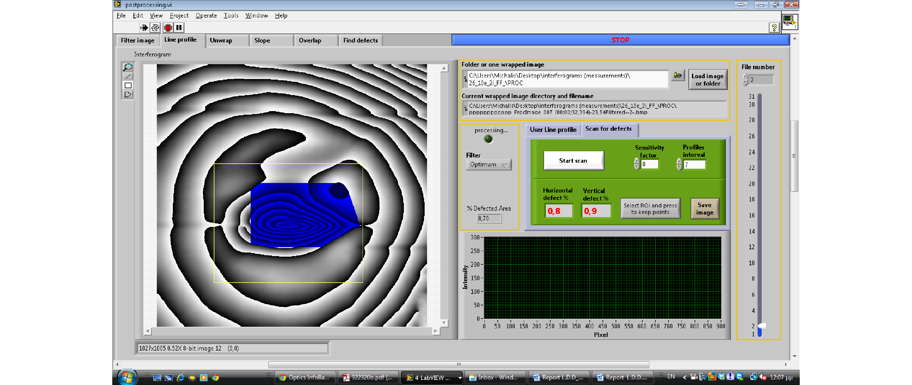
Fig. 14  Example of an automatic detection tool to extract partial field defects from whole-body fringes.

The example shows that part of the defect escaped detection, and it is likely that the algorithm will not identify all or may identify points that do not belong to the defect region; in this case, the operator can interactively correct the coordinates to fully assign the region. To optimize the software, further development is needed, with the aim of automatic detection in a number of sequential complex interferograms through additional algorithm clustering and K-means to better elaborate the defined defect areas. However, defect detection via automated software has been continuously disappointing in artwork structural diagnosis.

The following example shows an unknown stone sample investigation. The sample was homogeneously excited in a microwave oven for 15 min, and after exit from the oven, sequential interferograms were taken during the cooling down process at 10 s intervals. Fig. 15a shows an interferogram with its FFT, and Fig. 15b shows the details of the defect with its FFT. Although Fourier analysis can be utilized to generate a database of different materials with characteristic Fourier spectra, if sufficient samples of the same structural condition and aging are available, one can observe that these do not offer the required detailed information for the structural condition of the sample and the buried defect. Defect size, shape, location, defect morphology, defect coordinates, defect microstructure, and micromorphology, which can guide the conservator to apply protective measures and consolidation, are lost. Hence, the most essential information is not applicable for use in light of the conservation demand for the precise and accurate documentation of defect topography and the evaluation of structural conditions.

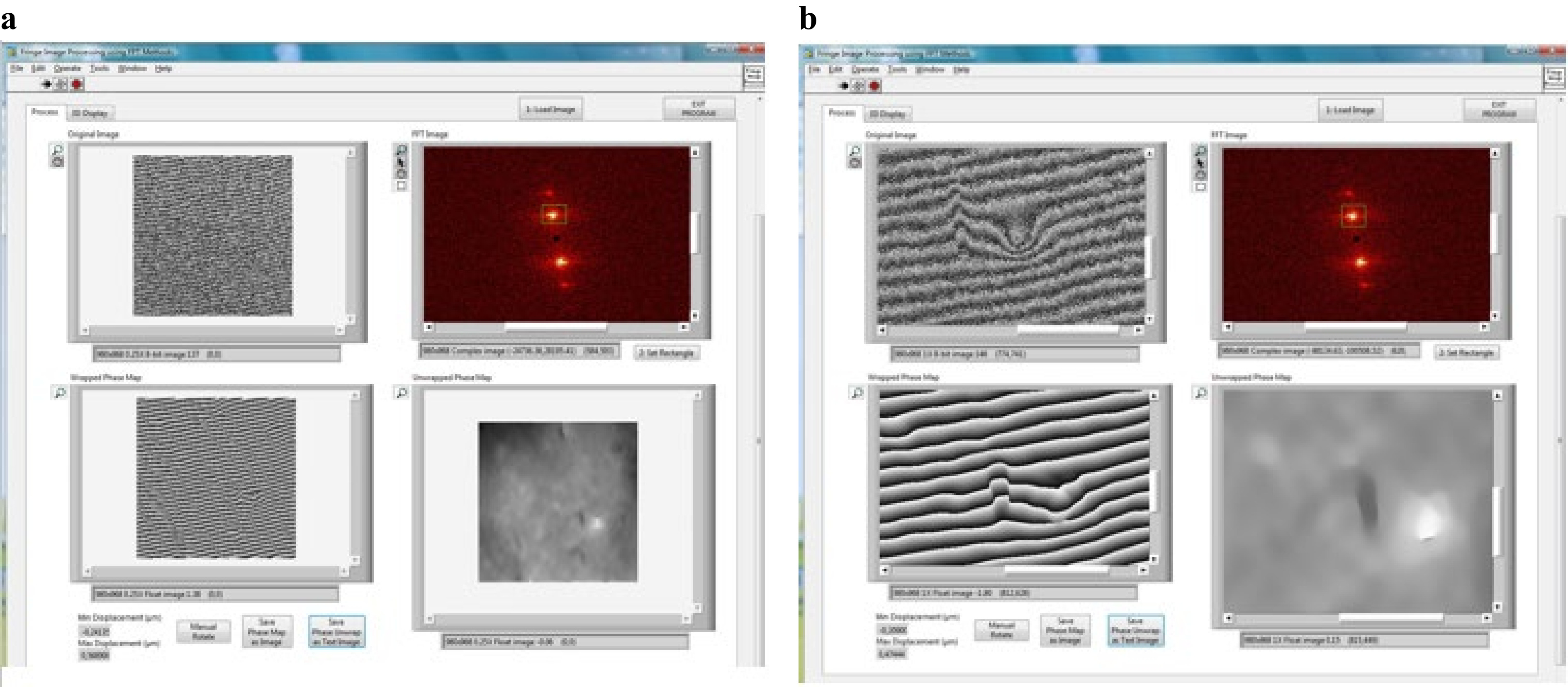
Fig. 15  Example of stone sample in a an interferogram of the whole surface of the sample and its FFT; b details of the defect and its FFT.

Automatic defect detection through wrapped interferograms has features that hold very important information to artwork conservation, but it poses a long-term challenge since it has been attempted in its fully traditional form in other applications via software tools without success or with very disappointing results with respect to artwork. The reason for this requires reference to the particular requirements of the structural diagnosis of artwork, especially the very nature of preventive application to aged artwork with a plethora of defects requiring analysis. In artwork conservation, any small defect may be important and crucial for structural integrity and long-term preservation. Defects should be described with information such as exact coordinates, shape and micromorphology, impact on surface, depth inside the bulk, type of defect, and relationship with other defects in order to provide a helpful diagnostic tool to ensure that protective interventions are properly applied.

Work is ongoing regarding this aspect.

In this paper it is described the conceptual path taken to support the evidential conclusion that fringe patterns exhibit scale-independent self-similarity and finally symmetry. They are stepwise described the experimental observations that paved the way to show the fringe pattern formation obeys symmetry laws, order and repeatability. Interference fringe patterns are manifestations of symmetry.

In this effort the aim is simple and straightforward based on the striking experimental data. The challenge and the future aim of the concept it is to develop algorithms capable of tracing automatically defects within complex fringe patterns. An advancement that could facilitate conservation and prevent deterioration of Cultural Heritage. Final aim is detection instruments based on high resolution measurements resolved by artificial intelligent supported algorithms for tracing and processing the information of interference fringe patterns which hold tremendous information worth exploring for conservation strategies and maintenance.

Holographic interferometry fringes provide reliable and accurate evidence of the surface displacement characterizing the condition of artwork. They are a valuable physical tool, even in cases of complex fringe formation, given their ability to facilitate direct structural diagnosis and evaluation. In this paper, we briefly present the methodology followed to first understand the significance of the main characteristics of fringe patterns, such as fringe density and fringe appearance, to detect physical reactions and defects in artwork based on raw interference fringe patterns before the unwrapping procedure. Unwrapping complex interferometric patterns, the most common result in artwork investigation using hologram interferometry-related techniques, can be very complex and impossible to accomplish via automatic software processing, as most methods fail to render important interferometric data useful to conservators, unless the data are unscrambled through external interaction and a priori knowledge of operator and then post-processed. In this context, instead of following the unwrapping and skeletonization method, we introduce and follow another path to accomplish direct visual evaluation through the study of the interference fringe characteristics of density and symmetry, as well as the study of secondary spatial frequency and the appearance of fringe patterns.

Research efforts are ongoing to accumulate the required knowledge of the reactions and effects that visualize and form interference fringes in artwork investigation to potentially facilitate know-how transfer and the development of algorithms for automated defect detection, localization, and isolation toward the delivery of an automatic defect detection process and automatic risk-index classification.

The unique holographic interferometry properties and image qualities that are only successfully formed and provided under strict boundary measuring conditions are the keys to a physically broader approach and understanding of the significance and utility of interferometry fringe patterns in art conservation, as opposed to strict technical approaches, as in most engineering disciplines, which result in less complex fringe patterns. Several physical analogies are employed to serve the specific objective of evaluating the problems encountered in structural diagnostics in the artwork field. The exhibited symmetry and its corresponding topology approach combined with the fringe density measurements can be implemented to deliver algorithms capable to deliver a direct defect topography map without losing information delivered by the interferogram. In this study, we proved the suitability of whole vs. partial field, surface topology geometries, and symmetry exhibited significance and evaluation. Implementing some or all of these physical analogies in the context of novel software development as approaches to deep learning and AI education may hold the key to automation. Research is ongoing.

I am grateful to my lab team and especially to my lab assistant, Michalis Andrianakis, as well as to all my colleagues throughout the years, co-authors and project partners, and especially the EC-funded projects LASERART, LASERACT, and MULTIENCODE, which allowed in-depth study of defect detection problems and ambiguities in the context of artwork. I would also like to acknowledge CLIMATE for CULTURE, which allowed further development of the monitoring of natural environmental effects.