


-
Over many years, imaging objects through random media has been a major technological challenge for many researchers1,2. This is because the techniques for imaging through random media constitute an essential common technological basis in a broad range of fields of science and technology, ranging from telescopic imaging through atmospheric turbulence in astronomy3 to microscopic imaging through scattering tissues in biology4. Reflecting the diversity and complexity of random media in the real world, a variety of techniques have been proposed to deal with the various characteristics of random media, as found in review articles5−9. To meet the scope of the special Anniversary Issue on Holography, this review places special emphasis on holographic techniques and their unique functionality, which play a pivotal role in imaging through random media. This review comprises two parts. The first part is intended to be a mini tutorial in which we first identify the nature of the problems encountered in imaging through random media. Through a methodological analysis, we then explain how the special functions that are unique to holography can be exploited to provide simple practical solutions to problems. In the second part, we introduce specific examples of experimental implementations and results based on different principles of holographic techniques, where the examples are taken from some of our recent work.
-
To understand the nature of the problem, let us first consider a simplified physical model to explain the way in which random media disturb imaging. For simplicity, we divide random media into two types based on their physical characteristics: inhomogeneous and scattering media for convenience of explanation. It should be noted that objects are not always outside the random medium, such as stars in astronomical imaging; they can be inside the random medium, such as cells in biomedical imaging, which makes the problem more complex. As illustrated in Fig. 1, the inhomogeneous medium is made of randomly distributed relatively mild refractive index variations on a macroscopic scale with a large spatial correlation length so that it remains transparent, such as heat shimmers caused by atmospheric refraction. Although the inhomogeneous medium introduces aberrations by distorting the wavefront of the light from an object, it preserves the validity of the concept of the wavefront defined for a bundle of rays of geometrical optics. On the other hand, the scattering medium is made of randomly distributed strong refractive-index variations at the microscopic scale with a short spatial correlation length. Incident light is scattered by the microstructure in the medium into many secondary wave components whose direction is determined by the phase function, creating a scrambled optical field that no longer has a well-defined wavefront in terms of geometrical optics. Thus, a typical scattering medium appears opaque, like ground glass.
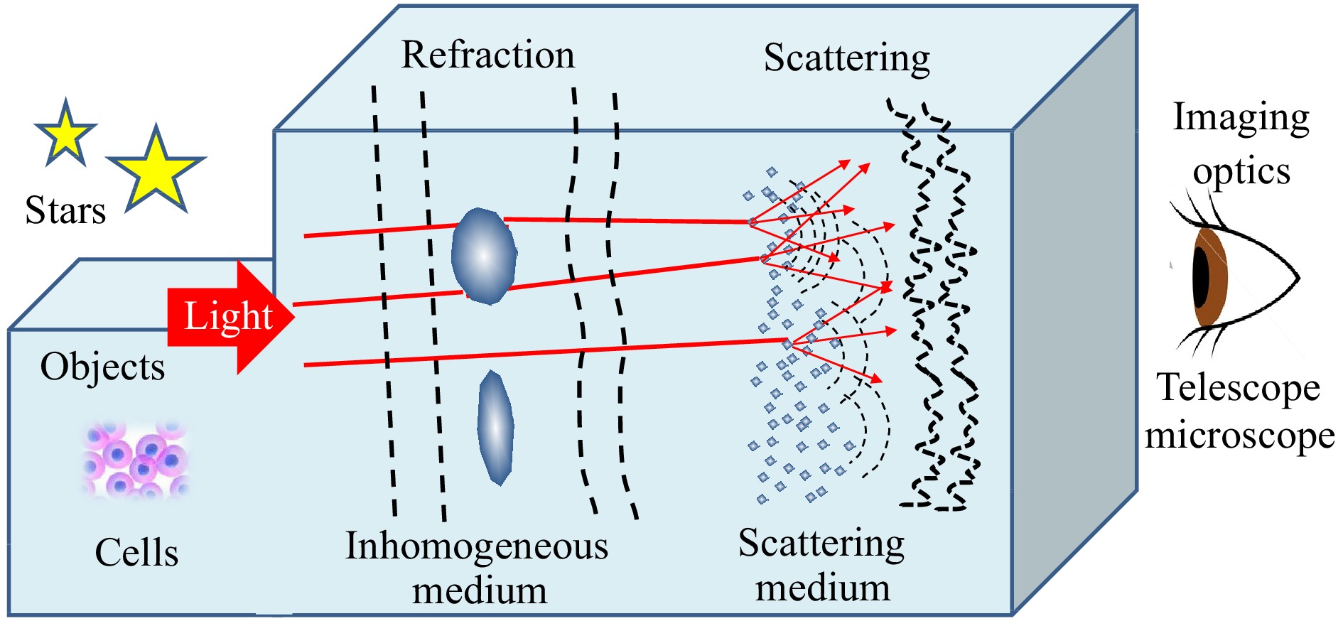
Fig. 1 Simplified model of random media with two typical physical characteristics.
In addition to the intrinsic physical properties of the media, its thickness has a significant influence on imaging performance. For example, with an increase in the thickness of a random medium, the shift invariance (i.e., isoplanatism or memory effect) of the imaging property tends to be lost. It is common to categorize scattering media into an optically thin scattering layer (e.g., ground glass) and a thick scattering volume (e.g., a tank of milk) according to the optical thickness (i.e., the number of scattering events occurring during light propagation). The concept of random media can be extended to include reflective optical surfaces, such as a randomly deformed mirror and a diffusely reflecting surface, which serve as an inhomogeneous medium and a scattering medium with extremely small thickness, respectively.
How random media disturb imaging depends not only on the characteristics of the random media, but also on their location between the object and the imaging optics. For example, ground glass severely disrupts the image when it is placed on the pupil plane of imaging optics, but it has a negligible influence when placed on the image plane to serve as a focus screen, such as a camera view finder.
It should also be noted that how the scale of the refractive index change in the media influences imaging performance is not determined by the geometric scale per se, but it is instead affected by its relative scale with respect to the imaging optics. For instance, the resolution of a ground telescope is determined by the relative scale of the correlation length of the atmospheric index changes (i.e., the Fried parameter) to the diameter of the telescope.
-
According to the simplified model of random media, the object light exiting from a random medium becomes a mixture of the three components, namely, unperturbed original light, non-scattered light with distorted wavefronts, and scattered light without well-defined wavefronts. The mixture ratio of the three components varies depending on the specific characteristics of the medium of interest. Because the problem arises from multiple sources of different natures, one must take a multifaceted approach to the problem. Here, we introduce the basic principles of the representative techniques and review them from a methodological viewpoint, with a particular focus on how the unique functionality of holography is effectively used in these techniques.
In the first step of searching for a solution to the problem, a choice can be made from the two options of the basic strategy: rejection or correction of bad light. The rejection strategy discriminates good light (unperturbed original light) from bad light (scattered light and aberrated light with distorted wavefronts) and rejects bad light in order only for good light to take part in imaging. Good light, however, is reduced rapidly as photons travel through the scattering medium, obeying Beer’s exponential law. The correction strategy does not reject bad light, but turns it into good light, so that nearly all light takes part in imaging. Holography plays a key role in both strategies and offers the additional merit of 3D imaging with full information of both amplitude and phase.
-
The best-known example of the rejection-based technique is optical coherence tomography10 (OCT), which rejects bad light and makes use of ballistic photons or unperturbed light that passes through the diffusive medium without being scattered. Ballistic photons take straight paths shorter than zigzags, followed by scattered photons. This difference in the light arrival time permits the discrimination between the good and bad light either by coherence gating with short temporal coherence light, as in OCT, with the low spatial coherence of light11, or by time gating using a short optical pulse, as with femto-photography12, in which the time-of-flight is detected with a streak camera. Since the early work of time gating by Duguay and Mattick13, various gating techniques14−16 have been proposed for rejecting scattered light.
Holography has an intrinsic gating function in its principle, per se. Specifically, the interference between the object and reference beams permits the reference beam to serve as a gating signal for time gating17, temporal coherence gating18, spatial coherence gating19, spatial frequency gating20, and Doppler-frequency-shift gating21,22. As illustrated in Fig. 2, an object hidden behind a scattering medium is recorded in a hologram using an ultrashort optical pulse or low-coherence continuous-wave (CW) light. Holographic recording occurs only when both the object and reference lights arrive at the recording point on the hologram precisely in synchronization within the time window set by the width of the light pulse or the coherence length of the CW light. Thus, by controlling the time delay of the reference light, one can set the desired time gate on the object light to be recorded on the hologram. For example, a series of time gates, spatially arranged in chronological order on the hologram, can be created by using a reference beam that illuminates the hologram at a grazing angle with its arrival time delay linearly mapped onto the spatial location on the hologram. This technique of time gating, known as light-in-flight recording17, enables the recording of high-speed holographic motion pictures of ultrafast phenomena. The time delay is introduced to the object beam not only by multiple scattering in the random medium, but also by the distance traveled by the object beam between the object and the hologram, which provides information about the object depth. Therefore, holographic time/coherence gating can be used for two purposes, namely, rejection of scattered lights, and tomographic sectioning of 3D objects, as in OCT.
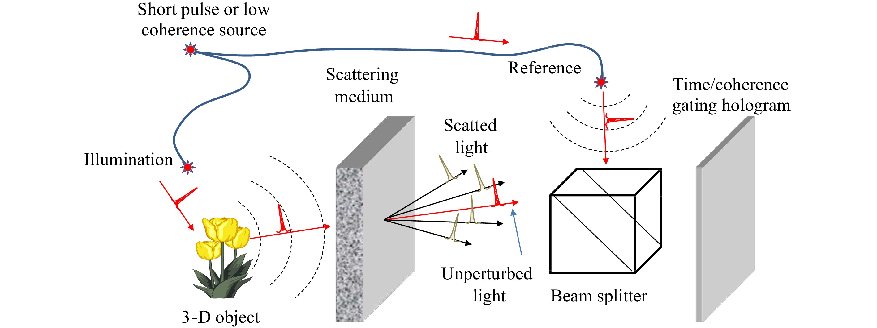
Fig. 2 Schematic illustration of the basic concept and principle of holographic time/coherence gating.
Although the technique of time/coherence gating is useful for rejecting multiple scattering light (and tomographic sectioning) with a large time delay, it cannot reject non-scattered aberrated lights (or snake photons) with distorted wavefronts. This is because the time delays corresponding to the wavefront aberrations of non-scattered light are too small to be discriminated by time/coherence gating, so that the aberrated light is accepted as good light. For this reason, wavefront aberration correction with adaptive optics is now one of the hot topics23 in OCT.
In addition to the limited rejection of aberrated light, the strategy of bad light rejection has a fundamental problem in that all useful information carried by the scattered and/or aberrated light is discarded, even though these bad light have more optical power than the good light in most random media. Therefore, an alternative strategy is necessary for this solution.
-
Before discussing holographic techniques, we begin with a quick overview of non-holographic techniques. A well-known example of the non-holographic technique for turning bad light into good light is adaptive optics24, in which an aberrated wavefront is detected with a wavefront sensor and corrected adaptively with a deformable mirror. With the advent of high-resolution spatial light modulators (SLMs) for phase modulation, various techniques for correcting distorted wavefronts with more complex phase structures have been demonstrated25,26. It should be noted, however, that adaptive optics works effectively only within a restricted field of view (i.e., the isoplanatic patch) over which the aberration does not change; in other words, the point spread function of the overall imaging system, including the random medium, retains shift invariance or isoplanatism. Astronomers are now making efforts to solve this problem using multi-conjugate adaptive optics27. A random medium is said to have a memory effect28 when its scattered field has a shift invariance with respect to the angle shift of the incident light. The memory effect is known to be closely related to the thickness of the random medium; a strongly scattering medium can have a memory effect as long as its scattering layer is thin (like ground glass), but it loses the memory effect as its thickness increases. The concept of the memory effect also plays an important role in other techniques, which is explained later.
Another type of non-holographic technique takes a mathematical approach to the problem, where the object information is retrieved numerically from the bad light by solving a sort of inverse problem in a wide sense. Specific techniques include model-based parametrization of the physical process for the solution search using optimization algorithms29−30, single-pixel imaging based on orthogonal pattern projection31,32, machine learning33, and neural networks34,35. These techniques are now enjoying rapid progress, and their success depends on how well the physical process and prior knowledge are integrated into the mathematical model.
-
The basic functions of adaptive optics (i.e., wavefront detection and correction) are included in the principle of holography. Wavefront detection is performed in the natural course of hologram recording because the hologram is nothing but an interferogram in which the wavefront,
${\phi _O}({\boldsymbol{r}})$ , of the object beam is recorded as$$ \begin{split} t({\boldsymbol{r}}) \propto & |{u_O}({\boldsymbol{r}}) + {u_R}({\boldsymbol{r}}){|^2}\; = \;|{u_O}({\boldsymbol{r}}){|^2} + 1 \\ & + |{u_O}({\boldsymbol{r}})|\exp [i{\phi _O}({\boldsymbol{r}})]\exp ( - i{\boldsymbol{k}} \cdot {\boldsymbol{r}}) \\ & + |{u_O}({\boldsymbol{r}})|\exp [ - i{\phi _O}({\boldsymbol{r}})]\exp (i{\boldsymbol{k}} \cdot {\boldsymbol{r}}) \end{split} $$ (1) where
$t({\boldsymbol{r}})$ is the amplitude transmittance of the hologram,${u_O}({\boldsymbol{r}})$ is the object beam, and${u_R}({\boldsymbol{r}})$ is the reference plane wave with a unit amplitude,$|{u_R}({\boldsymbol{r}})| = 1$ , and phase,${\phi _R} = {\boldsymbol{k}} \cdot {\boldsymbol{r}}$ , for off-axis holography. Also recorded in the hologram is the phase-conjugated object beam,${u_O}* = \;|{u_O}|\exp ( - i{\phi _O})$ , with the reversed sign of phase, which plays a key role in the wavefront correction, as explained below.As shown schematically in Fig. 3, the light from a coherently illuminated object is perturbed by a random medium and then recorded with a reference plane wave,
$\exp (i{\boldsymbol{k}} \cdot {\boldsymbol{r}})$ , in a hologram with the amplitude transmittance given by Eq. 1. When the hologram is read out with a counter-propagating plane wave,$\exp ( - i{\boldsymbol{k}} \cdot {\boldsymbol{r}})$ , a phase-conjugated object beam,${u_O}* = \;|{u_O}|\exp ( - i{\phi _O})$ , is generated from the last term in Eq. 1. Physically, it is a time-reversed object beam that propagates back into the random medium to retrace its path backward through it, like watching a time-reversed movie. As long as the time reversal symmetry holds with the physical law of wave propagation in the random medium, the light exiting from the random medium becomes the original unperturbed object light, although with the sign of phase reversed, which converges to form a real image of the object. Thus, bad light turned into good light.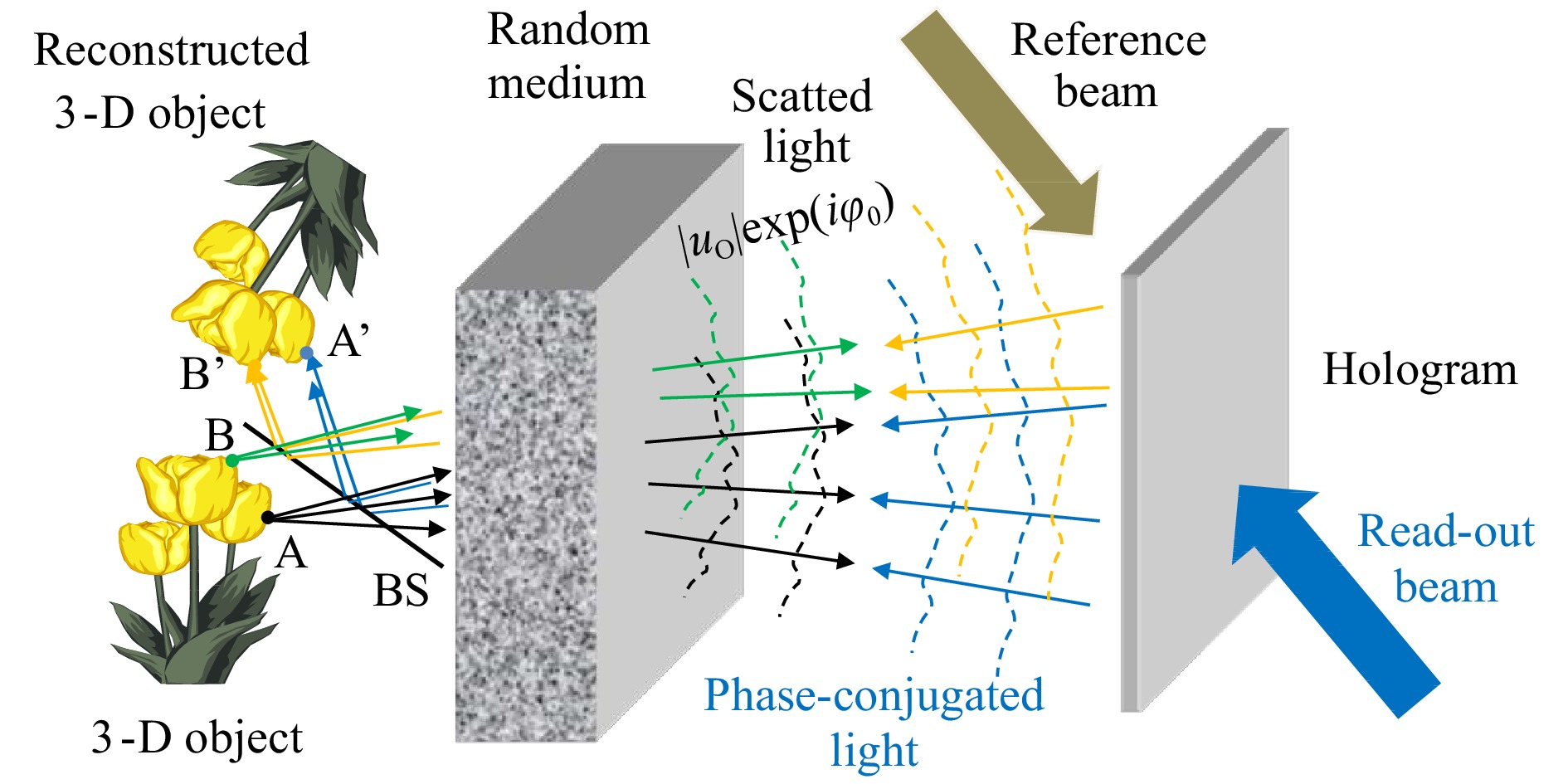
Fig. 3 Schematic illustration of the concept and principle of wavefront correction by holographic phase-conjugation.
The unique feature of holographic phase conjugation compared with adaptive optics is as follows. Referring to Fig. 3, we consider two points, A and B, at different locations on the object. The lights from these points as point sources (indicated by rays in black and green) pass through different parts of the random medium and receive different perturbations or wavefront distortions. In conventional adaptive optics, wavefront sensing is performed for a single point source (e.g., a guide star in astronomy), and wavefront correction is made for this single point in the field of view. This means that conventional adaptive optics cannot perform wavefront corrections simultaneously for points A and B from two isoplanatic patches with different perturbations. On the other hand, in holographic phase conjugation, every object point in the field of view serves as its own guide star for imaging itself with light backtracking through the random medium by virtue of time reversal. Therefore, holographic phase conjugation can have a wider field of view for thick and complex random media than conventional adaptive optics. Note, however, that because this advantage is brought about by the coherent holographic recording of objects, the technique of holographic phase conjugation cannot be applied directly to the imaging of incoherently illuminated objects, such as stars in astronomy and fluorescence-labeled cells in biology.
The technique of wavefront correction by holographic phase conjugation has a long history going back to early seminal work in the 1960s by Kogelnik36 and Leith and Upatnieks37. With the availability of novel holographic recording materials (e.g., photorefractive crystals) and high-resolution SLMs, new implementations of holographic phase conjugation have been proposed and demonstrated for imaging through random media, including optical phase conjugation using an Fe-doped LiNbO3 photorefractive crystals38, and a digital optical phase conjugation system39,40 based on the combination of a high-resolution image sensor and an SLM for digital wavefront sensing and correction.
-
The holographic phase conjugation described above requires duplication of the randomly perturbed object beam, with its phase sign reversed in the reconstruction process. It further requires precise alignment between the hologram and the random medium for the reconstructed phase-conjugated beam to precisely retrace the same path backwards through the random medium. Also, the corrected final image is not available downstream of the hologram, but is formed upstream of the original object itself; a solution to this third problem was given in Kogelnik and Pennington41.
In their seminal paper in 1966, Goodman et al. proposed yet another holographic technique42 (i.e., common-path holographic recording), which is free from the problems mentioned above. Fig. 4 shows the concept and principle of wavefront correction via quasi-common path holographic recording. For simplicity, the object is assumed to be a single point source at O on the object, although the principle applies to other points on the object. A reference point source is placed at point R, such that the distance, OR, between the object and reference points subtends a small field angle, θ, seen from a recording point, H, on the hologram. Suppose that the random medium is placed at distance, z, from the hologram, then the object and reference rays received at the recording point, H, have emerged from the random medium with relative lateral shift
$z\theta $ at the exit. Let Δ represent the lateral correlation length of the perturbed optical field exiting from the random medium, such that Δ is the average linear dimension over which the wavefront, emerging from the random medium, is nearly constant. If the angular distance between the object and the reference satisfies$\theta < \Delta /z$ , then the object and reference rays have passed through identical (i.e., highly correlated) portions of the random medium. In other words, it realizes a geometry for common-path holographic recording in which the common distortions of the reference and object waves cancel each other through interference. The condition,$\theta < \Delta /z$ , sets the maximum available field angle. Given a correlation length, Δ, (determined by the physical characteristic of the random medium), the field of view can be maximized for$z \approx 0$ by recording the hologram immediately behind the random medium. From the hologram recoded in this technique, the image can be reconstructed in the same manner as with a conventional hologram without special attention to alignment, and it can be observed downstream of the hologram.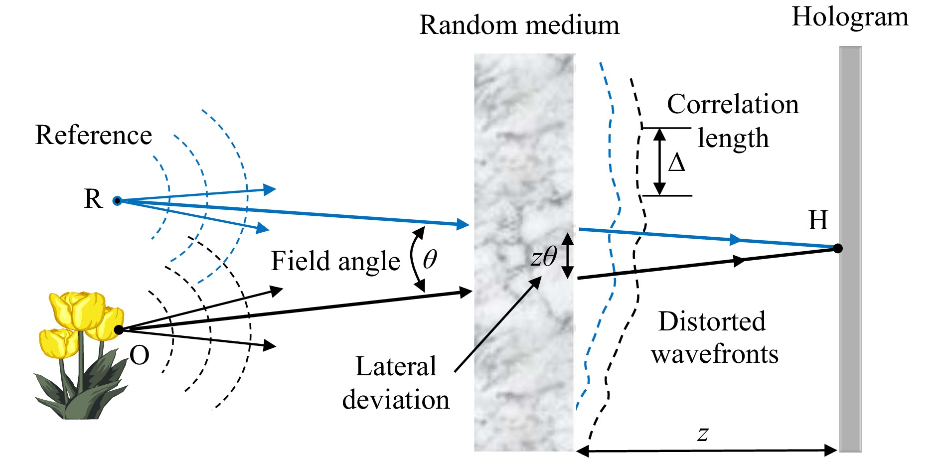
Fig. 4 Schematic illustration of the concept and principle of wavefront correction by common-path holographic recording.
After the early experimental demonstration of long-distance holographic imagery through air turbulence by Goodman et al.43, the concept and principle of common-path holographic recording were combined with digital holography to make new advancements44−46.
-
As preliminaries for the explanation of holographic correloscopy7, let us start with the principle of non-holographic imaging through a thin scattering medium based on speckle intensity correlation47,48. As shown in Fig. 5, the light from an object is scattered by a thin but strong scattering medium placed at a distance,
$\hat z$ , from the object, and the scattered field is observed on an observation plane at a distance, z, from the scattering medium. If the object is illuminated with spatially incoherent quasi-monochromatic light, and the scattering medium has a memory effect, the intensity distribution on the observation plane is given by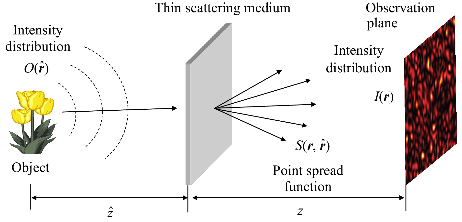
Fig. 5 Non-holographic imaging through a scattering medium based on speckle intensity correlation.
$$ I({\boldsymbol{r}}) = S({\boldsymbol{r}},{\boldsymbol{\hat r}}) * O({\boldsymbol{\hat r}}) = \int {S({\boldsymbol{r}} - {\boldsymbol{\hat r}})} \,O({\boldsymbol{\hat r}})d{\boldsymbol{\hat r}} $$ (2) where
$S({\boldsymbol{r}},{\boldsymbol{\hat r}})$ is the shift-invariant point spread function or the intensity speckle pattern created by a point source at point${\boldsymbol{\hat r}}$ on the object,$ O({\boldsymbol{\hat r}}) $ is the object intensity distribution, and$ * $ is the convolution operation with the angularly scaled coordinates,${\boldsymbol{r}} = z\,{\boldsymbol{\theta }}$ , and$ {\boldsymbol{\hat r}} = - \hat z\,{\boldsymbol{\theta }} $ ; the convolution represents the angular memory effect. We can now compute the autocorrelation of the observed intensity distribution.$$ \begin{split} I({\boldsymbol{r}}) \otimes I({\boldsymbol{r}}) = &\left[ {S({\boldsymbol{r}},{\boldsymbol{\hat r}}) * O({\boldsymbol{\hat r}})} \right] \otimes \left[ {S({\boldsymbol{r}},{\boldsymbol{\hat r}}) * O({\boldsymbol{\hat r}})} \right] \\ =& \left[ {S({\boldsymbol{r}},{\boldsymbol{\hat r}}) \otimes S({\boldsymbol{r}},{\boldsymbol{\hat r}})} \right] * \left[ {O({\boldsymbol{\hat r}}) \otimes O({\boldsymbol{\hat r}})} \right] \end{split} $$ (3) where
$ \otimes $ denotes autocorrelation; the passage to the second line of Eq. 3 can be easily confirmed from their relationship in the spectral domain. Remembering that$S({\boldsymbol{r}},{\boldsymbol{\hat r}})$ is the speckle pattern created by a point source at point${\boldsymbol{\hat r}}$ on the object, we note that$S({\boldsymbol{r}},{\boldsymbol{\hat r}}) \otimes S({\boldsymbol{r}},{\boldsymbol{\hat r}})$ has a sharp delta-correlation peak with its width corresponding to the average speckle size, which stands on a constant background resulting from the nonnegativity of$S({\boldsymbol{r}},{\boldsymbol{\hat r}})$ . By writing$$ S({\boldsymbol{r}},{\boldsymbol{\hat r}}) \otimes S({\boldsymbol{r}},{\boldsymbol{\hat r}}) \approx \delta ({\boldsymbol{\hat r}}) + {\rm{const}}. $$ (4) we obtain form Eq. 3,
$$ I({\boldsymbol{r}}) \otimes I({\boldsymbol{r}}) \approx O({\boldsymbol{\hat r}}) \otimes O({\boldsymbol{\hat r}}) + {\rm{const}}{\rm{. }} $$ (5) which states that, apart from the contrast reduction caused by the constant background, the intensity correlation of the scattered field gives the autocorrelation function of the intensity distribution of the hidden object. Hence, the remaining problem is determining the object intensity from its autocorrelation function. This is mathematically equivalent to the phase recovery problem of the power spectrum studied in the field of X-ray diffraction. Bertolotti et al.47 and Katz et al.48 used iterative phase-retrieval algorithms, such as the Fienup algorithm49, which make use of a priori knowledge about the object, as constraints in the solution search.
We are now ready to explain holographic correloscopy7,50 as another solution for phase recovery, remembering that holography was invented as a technique to preserve phase information that was lost by intensity recording in traditional photography. We add a reference point source at point
${{\boldsymbol{r}}_0}$ , as shown in Fig. 6, so that the intensity distribution in the object space becomes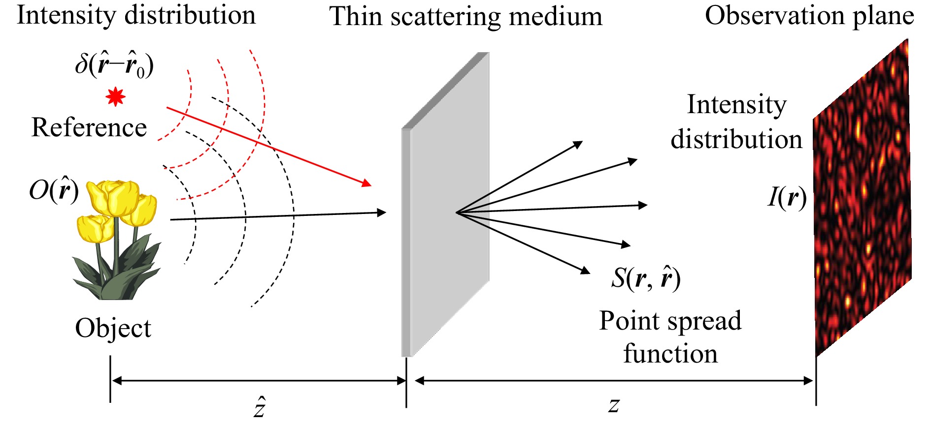
Fig. 6 Holographic correloscopy for imaging through a scattering medium based on speckle intensity correlation.
$$ {I_O}({\boldsymbol{\hat r}}) = O({\boldsymbol{\hat r}}) + \delta ({\boldsymbol{\hat r}} - {{\boldsymbol{\hat r}}_0}) $$ (6) Note that this is the intensity distribution under spatially incoherent illumination, and it differs from the familiar complex amplitude distribution of coherent illumination, such as that shown in Fig. 4. Replacing
$ O({\boldsymbol{\hat r}}) $ in Eq. 5 with${I_O}({\boldsymbol{\hat r}})$ , we have$$ \begin{split} I({\boldsymbol{r}}) \otimes I({\boldsymbol{r}}) \approx &\left[ {O({\boldsymbol{\hat r}}) + \delta ({\boldsymbol{\hat r}} - {{{\boldsymbol{\hat r}}}_0})} \right] \otimes \left[ {O({\boldsymbol{\hat r}}) + \delta ({\boldsymbol{\hat r}} - {{{\boldsymbol{\hat r}}}_0})} \right] + {\rm{const}}. \\ \approx & O({\boldsymbol{\hat r}} + {{{\boldsymbol{\hat r}}}_0}) + O\left( { - ({\boldsymbol{\hat r}} - {{{\boldsymbol{\hat r}}}_0})} \right) \\&+ O({\boldsymbol{\hat r}}) \otimes O({\boldsymbol{\hat r}}) + \delta ({\boldsymbol{\hat r}}) + {\rm{const.}} \\[-10pt] \end{split} $$ (7) As in conventional holography, the first term,
$ O({\boldsymbol{\hat r}} + {{\boldsymbol{\hat r}}_0}) $ , gives a laterally shifted image of the object, whereas the second term,$ O( - ({\boldsymbol{\hat r}} - {{\boldsymbol{\hat r}}_0})) $ , gives a symmetrically shifted image. We regard the remaining terms as noise appearing in the center and background. Thus, we can reconstruct the image using speckle intensity correlation. Singh et al.50 demonstrated full 3D holographic correloscopy by making use of the memory effect in the axial direction.Eq. 7 suggests that the real essence of the principle lies in the cross-correlation term between the object and reference,
$ \delta ({\boldsymbol{\hat r}} - {{\boldsymbol{\hat r}}_0}) \otimes O({\boldsymbol{\hat r}}) $ , which generates the original image corresponding to the interference between the reference and object beams in conventional holography. Then, an idea naturally arises that we record the speckle pattern,$ S({\boldsymbol{r}},{\boldsymbol{\hat r}}) $ , or the point spread function, in advance with a reference point source only. We would then compute its cross-correlation with the speckle pattern,$ I({\boldsymbol{r}}) $ , of the object:$$ \begin{split} S({\boldsymbol{r}},{\boldsymbol{\hat r}}) \otimes I({\boldsymbol{r}}) =& S({\boldsymbol{r}},{\boldsymbol{\hat r}}) \otimes \left[ {S({\boldsymbol{r}},{\boldsymbol{\hat r}}) * O({\boldsymbol{\hat r}})} \right] \\ = &\left[ {S({\boldsymbol{r}},{\boldsymbol{\hat r}}) \otimes S({\boldsymbol{r}},{\boldsymbol{\hat r}})} \right] * O({\boldsymbol{\hat r}})\\ \approx & O({\boldsymbol{\hat r}}) + {\rm{const}}. \end{split} $$ (8) where use is made of the relation in Eq. 4. In fact, this idea was devised by Freund51 in 1990 in his seminal paper on wall lens, which largely influenced recent research in scatter-based lensless microscopy52. This cross-correlation technique requires two steps of speckle recording; therefore, it is not suitable for imaging through dynamic random media, but it has the advantage of removing noise terms. The principles explained so far are based on intensity correlation under spatially incoherent illumination. Next, we consider the case of a field correlation under coherent illumination.
Referring to Fig. 6, a similar discussion can be made by replacing the intensity variables (denoted by uppercase letters) with the complex-amplitude variables (denoted by the corresponding lowercase letters, apart from the field on the observation plane denoted by
$u({\boldsymbol{r}})$ ). Assuming the memory effect, the complex field on the observation plane is given by$$ u({\boldsymbol{r}}) = s({\boldsymbol{r}},{\boldsymbol{\hat r}}) * {u_O}({\boldsymbol{\hat r}}) $$ (9) where
$s({\boldsymbol{r}},{\boldsymbol{\hat r}})$ is the amplitude point spread function, and${u_O}({\boldsymbol{\hat r}})$ is the field resulting from the superposition of the object and the reference point source.$$ {u_O}({\boldsymbol{\hat r}}) = o({\boldsymbol{\hat r}}) + \delta ({\boldsymbol{\hat r}} - {{\boldsymbol{\hat r}}_0}) $$ (10) The autocorrelation function (i.e., the spatial coherence function) of the field on the observation plane is given by
$$ \begin{split} \Gamma ({\boldsymbol{r}}) =& u({\boldsymbol{r}}) \otimes u({\boldsymbol{r}}) \\ =& \left[ {s({\boldsymbol{r}},{\boldsymbol{\hat r}}) * {u_O}({\boldsymbol{\hat r}})} \right] \otimes \left[ {s({\boldsymbol{r}},{\boldsymbol{\hat r}}) * {u_O}({\boldsymbol{\hat r}})} \right] \\ =& \left[ {s({\boldsymbol{r}},{\boldsymbol{\hat r}}) \otimes s({\boldsymbol{r}},{\boldsymbol{\hat r}})} \right] * \left[ {{u_O}({\boldsymbol{\hat r}}) \otimes {u_O}({\boldsymbol{\hat r}})} \right] \\ \end{split} $$ (11) An important difference from the previous intensity case is that the autocorrelation of the complex-valued speckle field does not have an unwanted constant background.
$$ s({\boldsymbol{r}},{\boldsymbol{\hat r}}) \otimes s({\boldsymbol{r}},{\boldsymbol{\hat r}}) \approx \delta ({\boldsymbol{\hat r}}) $$ (12) so that we have from Eqs. 10,11,
$$ \begin{split} \Gamma ({\boldsymbol{r}}) \approx & \left[ {o({\boldsymbol{\hat r}}) + \delta ({\boldsymbol{\hat r}} - {{{\boldsymbol{\hat r}}}_0})} \right] \otimes \left[ {o({\boldsymbol{\hat r}}) + \delta ({\boldsymbol{\hat r}} - {{{\boldsymbol{\hat r}}}_0})} \right] \\ \approx & \,o({\boldsymbol{\hat r}} + {{{\boldsymbol{\hat r}}}_0}) + o\left( { - ({\boldsymbol{\hat r}} - {{{\boldsymbol{\hat r}}}_0})} \right) + o({\boldsymbol{\hat r}}) \otimes o({\boldsymbol{\hat r}}) + \delta ({\boldsymbol{\hat r}}) \end{split} $$ (13) Thus, the object hidden behind the scattering medium can be reconstructed from the spatial coherence function of the scattered optical field. The most important difference from the intensity correlation is that we can reconstruct the complex amplitude of the object, including the phase information, which permits the holographic interferometry of an object hidden behind the scattering medium44.
So far, the principle of correloscopy has been explained without providing a clear explanation of the definition of the correlation operation denoted by
$ \otimes $ . Mathematically, the correlation between statistical signals is defined using the ensemble average as$g({\boldsymbol{r}}) \otimes g({\boldsymbol{r}}) = < g({\boldsymbol{r}}' + {\boldsymbol{r}})g^*({\boldsymbol{r}}') > $ . In practice, however, the ensemble average, <…>, needs to be replaced either by the temporal average or by the spatial average, assuming the stationarity of the statistical process53. Although the temporal average is suitable for imaging with time-varying speckle fields through a dynamic scattering medium, such as rotating ground glass, the spatial average is used in imaging through a static scattering medium, as is often the case with speckle intensity correlation.Here, we show two different ways to implement the principle of field-correlation correloscopy. Fig. 7 shows an example of a fully optical implementation based on a shearing interferometer. The spatial coherence function of the scattered field is detected and visualized in real time as the contrast and shift of interference fringes using a radial shearing interferometer54. This scheme, which originated from coherence holography55, is suitable for imaging through a dynamic scattering medium that permits spatial coherence detection through the time averaging of the speckle fields with the image sensor as an integrator.
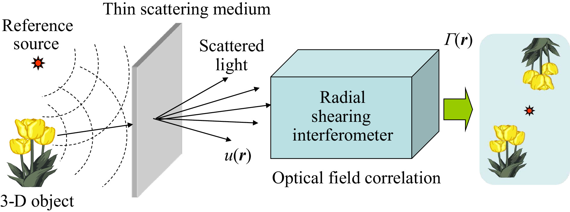
Fig. 7 Interferometric implementation of holographic correloscopy for imaging through a scattering medium.
For the case of a dynamic scattering medium, such as rotating ground glass, we can find a much simpler solution than the interferometric implementation (shown in Fig. 7) in which the coherence function,
$\Gamma ({\boldsymbol{r}})$ , of the scattered field was detected on the observation plane, so as to follow the result in Eq. 13. Let us first note that the thin but strong scattering medium in fast motion destroys the coherence of both the object and the reference beams and serves as a spatially incoherent extended source with the light intensity distribution,${I_S}({\boldsymbol{\tilde r}})$ . Next, let us note further that, from the van Cittert-Zernike theorem1, the coherence function of the scattered field,$\Gamma ({\boldsymbol{r}})$ , can be obtained from the Fourier transform of the incoherent source intensity distribution,${I_S}({\boldsymbol{\tilde r}})$ . Now, we have reached a simpler solution44. Instead of detecting the coherence function, we detect the intensity distribution of the field exiting the scattering medium by using imaging optics focused on the scatter surface, as illustrated in Fig. 8. Because the scatter medium is thin, the intensity distribution,${I_S}({\boldsymbol{\tilde r}})$ , represents the lensless Fourier transform hologram created by the object and point source. Hence, we can understand, without knowledge of the van Cittert-Zernike theorem, that the object can be reconstructed by computing the inverse Fourier transform of the intensity distribution,${I_S}({\boldsymbol{\tilde r}})$ , detected with an image sensor; the time-averaged operation takes place over one frame period of the image sensor, which averages out speckles.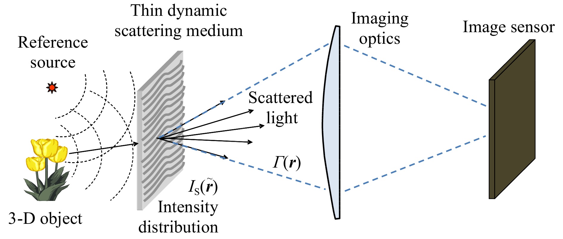
Fig. 8 Simpler implementation of holographic correloscopy for imaging through a scattering medium.
It is of interest to note that this simple implementation (remote imaging digital holography7) of holographic correloscopy can be interpreted as an extreme case of common-path holography (shown in Fig. 4), in which the locations of the random medium and hologram are identical with
$z = 0$ , so that the perfect common-path geometry is realized. -
To provide an idea of how the principles explained in the previous sections are implemented in actual physical systems, we next introduce some specific examples from our past work alongside experimental results.
-
Fig. 9 shows a specific example of a fully optical implementation of holographic correloscopy by Naik et al.54, which corresponds to the principle illustrated in Fig. 7. The optical setup at the top of Fig. 9a creates a lensless Fourier transform hologram of an object pattern, UEC, on a rotating ground glass, which hinders direct observation of the object through it. The light scattered from the ground glass was introduced into a Sagnac radial shearing interferometer, which functions as a real-time optical field correlator that visualizes the complex-valued spatial coherence function directly in the form of the fringe contrast and the fringe shift, as shown in Fig. 9b. The reconstructed image of the hidden object was quantified by fringe analysis, as shown in Fig. 9c.
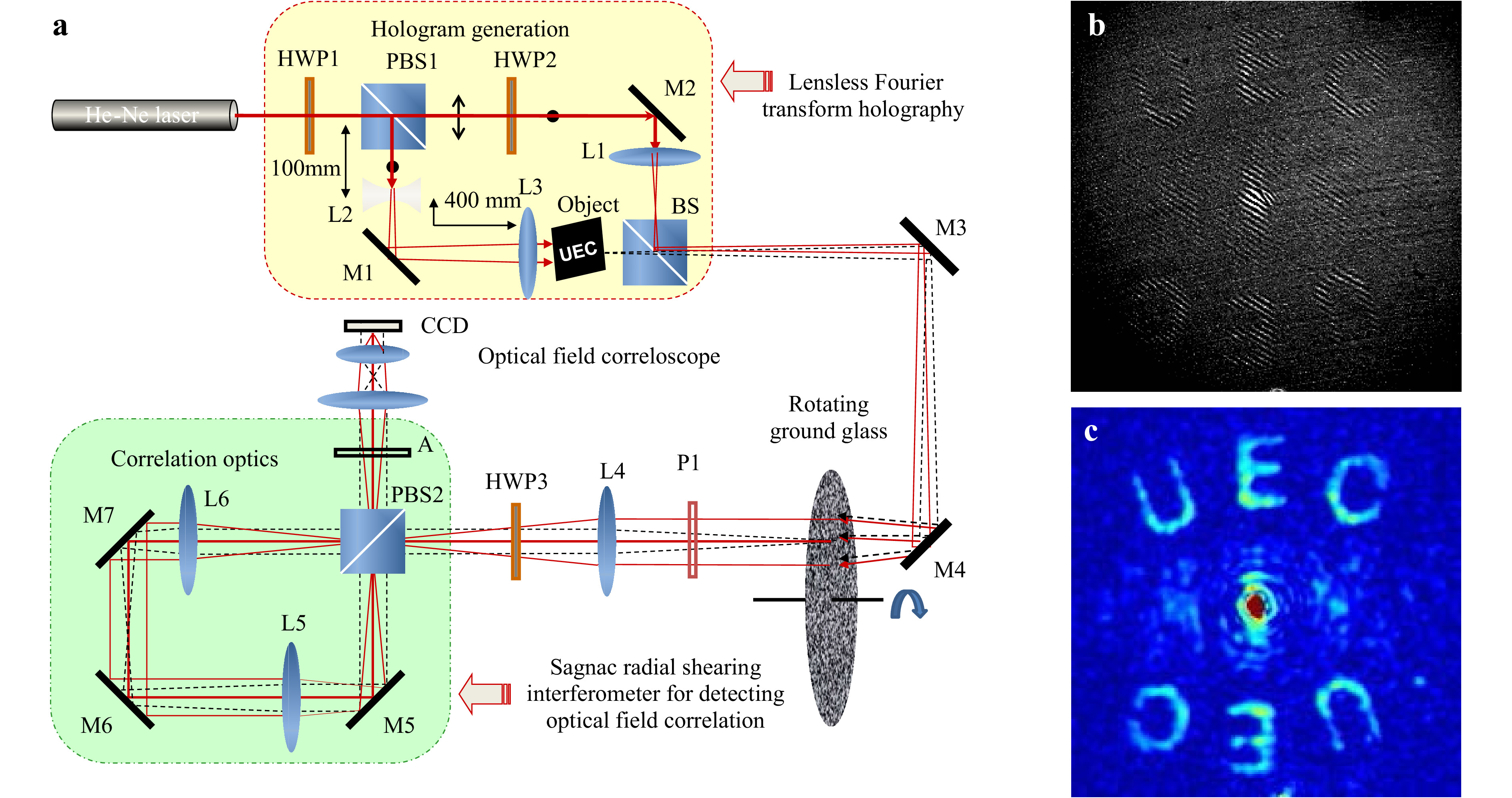
Fig. 9 Holographic correloscopy based on field correlation with a radial shearing interferometer54. a Experimental setup. b Raw fringe pattern. c Fringe contrast (modulus of coherence function). Reproduced with permission from OSA. ©OSA
-
Fig. 10 shows an example of the remote imaging digital holography proposed by Singh et al.44 for imaging through a dynamic scattering medium. The photo in Fig. 10a shows the experimental setup for implementing the scheme illustrated in Fig. 8. Fig. 10b shows a magnified view of an object and a reference point source, which creates a lensless Fourier transform hologram on a rotating diffuser. Although the rotating diffuser hides the object from the camera, it permits the intensity distribution of the hologram on the diffuser to be imaged by the camera onto a high-resolution CCD image sensor, which also functions as a time integrator to average out speckles during one frame period to capture the hologram. In Fig. 10, (c) shows the hidden object reconstructed from the hologram, and (d) demonstrates the holographic interferometry of the hidden object, in which the left and right photographs show, respectively, the amplitude and phase of the object under thermal deformation for holographic interferometry.
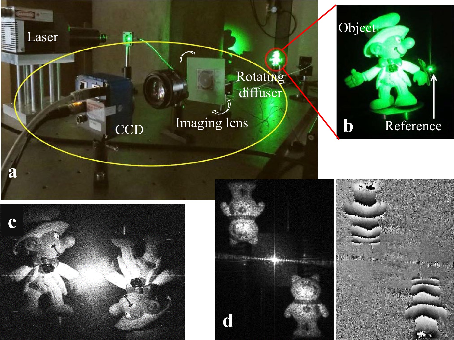
Fig. 10 Remote imaging digital holography for imaging through a dynamic scattering medium44. a Experimental setup. b Magnified view of an object and a reference source. c Reconstruction of the hidden object. d Holographic interferometry of the hidden object. Reproduced with permission from OSA. ©OSA
-
Fig. 11 shows an example of the experimental results obtained by Singh et al.50 using the principle of holographic correloscopy based on the speckle intensity correlation shown in Fig. 6. Fig. 11a shows a microscope image of an original object (a USAF test target), which was placed together with a reference point source at a location hidden behind a diffuser and illuminated with spatially incoherent quasi-monochromatic light. Fig. 11b shows the auto-covariance (i.e., the autocorrelation with the average subtracted) of the speckle intensity of the light scattered by the diffuser. Note the small twin images reconstructed in the top-left and bottom-right corners in symmetry to the central block, stopping the strong central correlation peak. Fig. 11c shows a magnified view of the reconstructed image of the object hidden behind the diffuser. The images in Fig. 11, from (d) through (g), demonstrate imaging through a biological sample (a 1.5-mm-thick chicken breast tissue), where (d) is an original object pattern “H” hidden behind the biological sample, (e) the speckle intensity distribution of the light scattered from the tissue, (f) the auto-covariance of the speckle pattern with the twin images of “H” being reconstructed in the corners, and its magnified image is shown in (g).
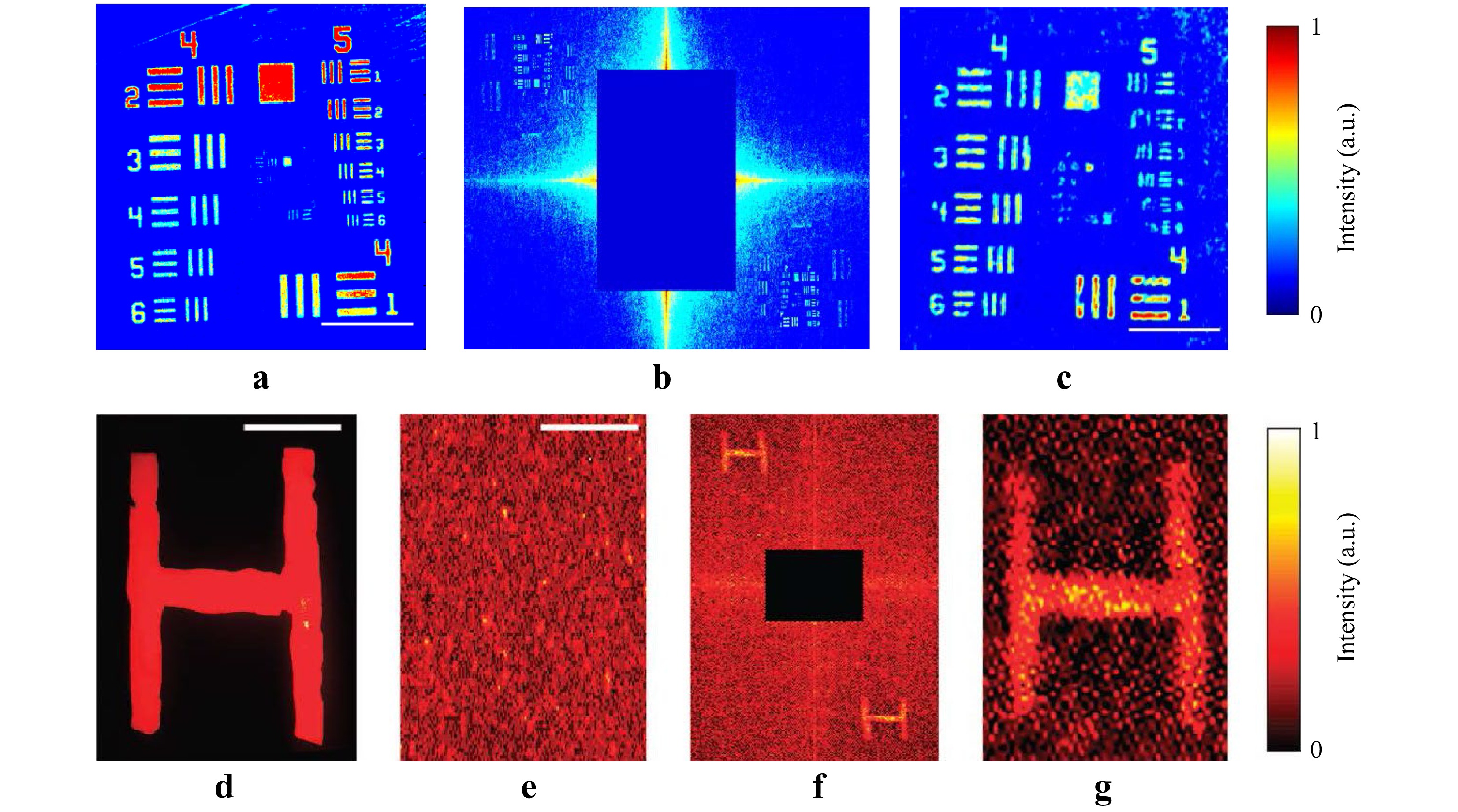
Fig. 11 Experimental results of holographic correloscopy based on speckle intensity correlation50. a Original object. b Auto-covariance of speckle intensity pattern with its central correlation peak blocked. c Reconstructed object. d Original object. e Speckle intensity of light scattered by biological tissue. f Auto-covariance of speckle intensity pattern with its central correlation peak blocked. g Reconstructed object. Reproduced with permission from Springer Nature. © Springer Nature
-
The concept of Freund’s wall lens51, based on the cross-correlation between the speckle point spread function and the speckle intensity distribution from an object, as in Eq. 8, was extended by Singh et al.52 to give rise to a scatterplate microscope that makes full use of the magnification property of the memory effect28,51.
As shown in Fig. 12, a traditional microscope has an objective lens that forms sharp images of a point source and an object, as shown in (a) and (b). If we replace the objective lens with a thin scatter plate, we have a point spread speckle pattern, as shown in (c) and an object speckle pattern, as shown in (d). Because of the angular shift invariance of the memory effect, a shift of the point source on the object space results in a corresponding shift in the speckle pattern magnified by
$m = - z/\hat z$ times; thus, the scatter plate can serve as a scattering microscope if the original object image is retrieved from the intensity cross-correlation between the two scattered fields shown in (c) and (d). In Fig. 12, (e) is an original object, the numeral 6, (f) the point spread speckle pattern of the scatter plate, (g) the object intensity speckle pattern, and (h) is the image reconstructed from the cross-correlation between the speckle patterns in (f) and (g). Figs. 12i−k demonstrate the application of the scatter-plate microscope to a biological sample (a section of a pine wood stem). In Fig. 12, (i) and (j) are images observed with a conventional microscope (NA = 0.16) illuminated with monochromatic and white light, respectively, and (k) is the image obtained with the scatter-plate microscope (NA = 0.16); the scale bar in the bottom right is 20 µm.
Fig. 12 Scatter-plate microscope based on speckle intensity cross-correlation52. a Point spread function of microscope. b Image of microscope. c Point spread function of scatter plate. d Scattered object light. e Object. f Point spread function of scatter plate. g Scattered object light. h Reconstructed object. i Monochromatic microscope image. j White-light microscope image. k Reconstructed scatter-plate image. Reproduced with permission from Springer Nature. © Springer Nature
-
Although remote imaging digital holography44 in Fig. 10 has the advantage of reconstructing the complex field (including phase information) of an object hidden behind a random medium, its application is limited to a dynamic scattering medium. Kodama et al.45 proposed a scheme for in-line phase-shift digital holography that can image through a static scattering medium. Illustrated in Fig. 13a is an experimental setup in which the light from an object, O, and the phase-shifted reference light are superposed in line to create broad holographic fringes on the static scattering medium, S, as shown in the inset. Because the in-line holographic fringes with no spatial carrier frequency are much broader than the scale of subjective speckles caused by the finite aperture of the imaging lens L on the scatter medium, the hologram is robust to subjective speckle noise. Therefore, in-line phase-shift digital holography permits reconstruction of the image without time averaging the speckles introduced by the scattering medium. Fig. 13b shows a demonstration of the 3D imaging through a static scattering medium. A 3D object is made of a bead (for phase object) and a grid pattern (for amplitude object) placed 1.32-mm apart from each other, and its 3D image was reconstructed numerically by moving the focal plane, as shown in the middle. The figures at the bottom of Fig. 13b show the grid pattern (left) and the bead (right) in focus. Quantitative phase imaging was also realized by submerging the beads in an index-matched liquid. Fig. 13c demonstrates imaging a test chart through a shaved rat skin with a thickness ~0.5 mm (shown in top). The bottom picture shows the reconstructed image of the test chart hidden behind the rat skin.
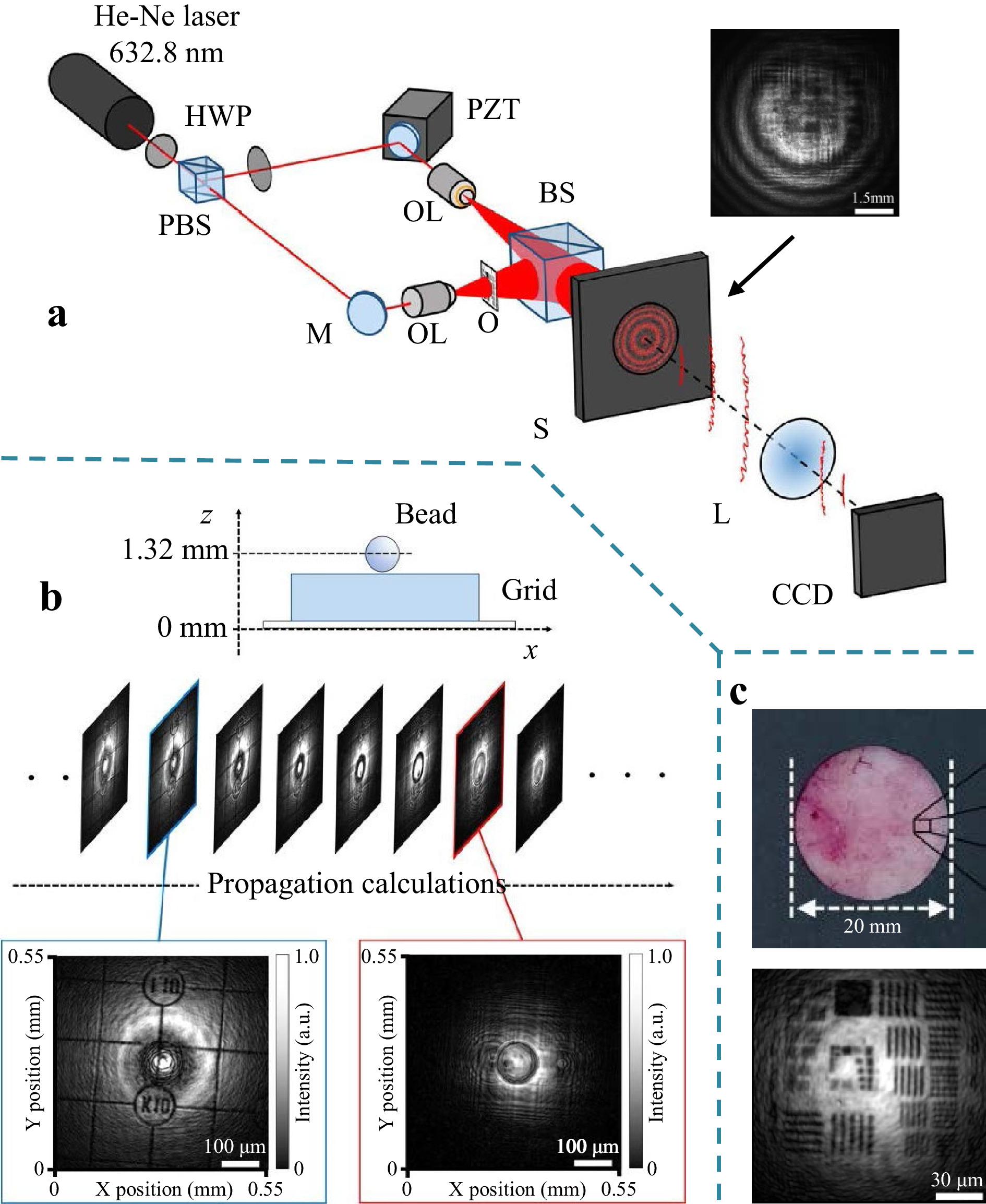
Fig. 13 Imaging through scattering media based on in-line phase-shift digital holography45. a Experimental setup. b Imaging 3-D object through a diffuser. c Imaging a test chart though a rat skin. Reproduced with permission from OSA. © OSA.
-
Attempts are now being made to explore the possibility of imaging through an inhomogeneous medium with increased thickness using common-path holographic recording (shown in Fig. 4). Fig. 14 shows an example of numerical experiments conducted by Kodama et al.46 A thick 3D inhomogeneous medium was modeled as a sequence of multiple thin layers with inhomogeneous refractive index distributions. As shown at the top of Fig. 14, 10 inhomogeneous layers were placed at depths z = 0.1~1.0 mm in the optical path with a separation of 0.1 mm between layers. Each layer introduces phase fluctuations over the range [0, 2π] with a spatial correlation generated by low-pass filtering (see bottom left in Fig. 14). The object and reference beams passed through the 10 layers with a relative angle of θ=1°; thus, the common-path condition,
$\theta \leqslant \Delta /z$ , (see Fig. 4) is satisfied for all layers in the inhomogeneous medium. Referring to the three framed pictures at the bottom of Fig. 14, the left shows the image reconstructed without the inhomogeneous medium, and the center and the right show, respectively, the image reconstructed by the conventional (non-common path) digital holography technique and the image reconstructed by the proposed common-path digital holography technique. This shows that common-path holographic recording is promising. At the time of this writing, the efficacy of common-path holographic recording for imaging through a thick and complicated heterogeneous medium has been confirmed experimentally57.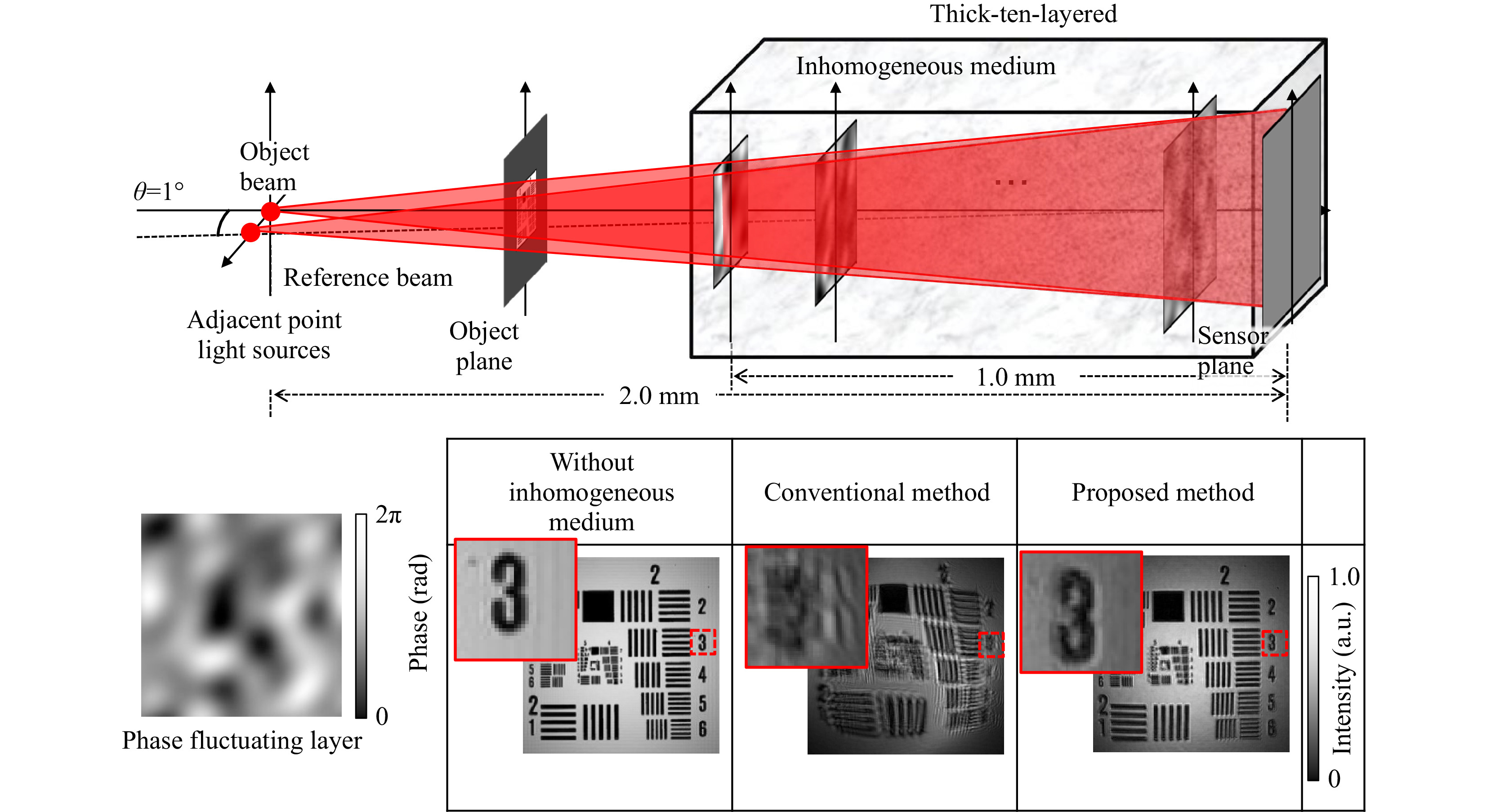
Fig. 14 Imaging through thick inhomogeneous medium by common-path holographic recording; a numerical experiment46. Reproduced with permission from OSA. © OSA.
-
We have reviewed the principles and techniques for imaging through random media, with a special focus on holographic techniques to meet the scope of the special Anniversary Issue on Holography. Although we have seen how the potential of holography has been exploited from past to present, there still remain many technological challenges for future topics in this research field, such as polarization imaging through birefringent random media, including the vectorial nature of optical fields, and multi-spectral color imaging through dispersive random media. One of the potential solutions may be found in the interdisciplinary integration of physics and informatics, such as in the marriage between optics/photonics and artificial intelligence56, which is already in progress33−35.
This paper is not intended to provide a comprehensive, balanced review. Rather, we presented our own view of the similarities and differences of the basic principles of various imaging techniques through random media. This is particularly applicable to the mini-tutorial in the first part of the review, in which we did not necessarily explain the principles in the same way as they were explained in the original papers. This choice was made just for our interest in identifying hidden links between different techniques, but we hope that it will also be of interest to the reader. The second part was to introduce part of the joint efforts made in this field by three universities: Universität Stuttgart (ITO), the University of Electro-Communications (UEC, Tokyo), and Utsunomiya University (CORE). The authors are grateful to all the members who have joined our joint endeavors.
-
E. Watanabe acknowledges support from a Grant-in-Aid for Transformative Research Areas(A) Grant Number A20H05888.
Holographic 3D Imaging through Random Media: Methodologies and Challenges
-
Mitsuo Takeda1, *, ,
 ,
, - Wolfgang Osten2,
-
Eriko Watanabe3, *, ,
- Light: Advanced Manufacturing 3, Article number: (2022)
- Received: 09 September 2021
- Revised: 26 January 2022
- Accepted: 08 February 2022 Published online: 01 May 2022
doi: https://doi.org/10.37188/lam.2022.014
Abstract: Imaging through random media continues to be a challenging problem of crucial importance in a wide range of fields of science and technology, ranging from telescopic imaging through atmospheric turbulence in astronomy to microscopic imaging through scattering tissues in biology. To meet the scope of this anniversary issue in holography, this review places a special focus on holographic techniques and their unique functionality, which play a pivotal role in imaging through random media. This review comprises two parts. The first part is intended to be a mini tutorial in which we first identify the true nature of the problems encountered in imaging through random media. We then explain through a methodological analysis how unique functions of holography can be exploited to provide practical solutions to problems. The second part introduces specific examples of experimental implementations for different principles of holographic techniques, along with their performance results, which were taken from some of our recent work.
Research Summary
Holographic 3D imaging through random media: Holography unveils hidden objects
Imaging through random media is a challenging problem of crucial importance in a wide range of fields of science and technology, ranging from telescopic imaging through atmospheric turbulence in astronomy to microscopic imaging through scattering tissues in biology. Mitsuo Takeda from Utsunomiya University, Wolfgang Osten from Stuttgart University, and Eriko Watanabe from the University of Electro-Communications review principles and techniques for holographic imaging through random media. First, the true nature of the problems encountered in imaging through random media is identified. Then, through a methodological analysis, how unique functions of holography can be exploited to provide practical solutions to problems is explained. Specific examples of experimental implementations for different principles of holographic techniques, along with their performance results, are introduced.


Rights and permissions
Open Access This article is licensed under a Creative Commons Attribution 4.0 International License, which permits use, sharing, adaptation, distribution and reproduction in any medium or format, as long as you give appropriate credit to the original author(s) and the source, provide a link to the Creative Commons license, and indicate if changes were made. The images or other third party material in this article are included in the article′s Creative Commons license, unless indicated otherwise in a credit line to the material. If material is not included in the article′s Creative Commons license and your intended use is not permitted by statutory regulation or exceeds the permitted use, you will need to obtain permission directly from the copyright holder. To view a copy of this license, visit http://creativecommons.org/licenses/by/4.0/.

 DownLoad: