Deterministic form-position deflectometric measurement of monolithic multi-freeform optical structures via Bayesian multisensor fusion

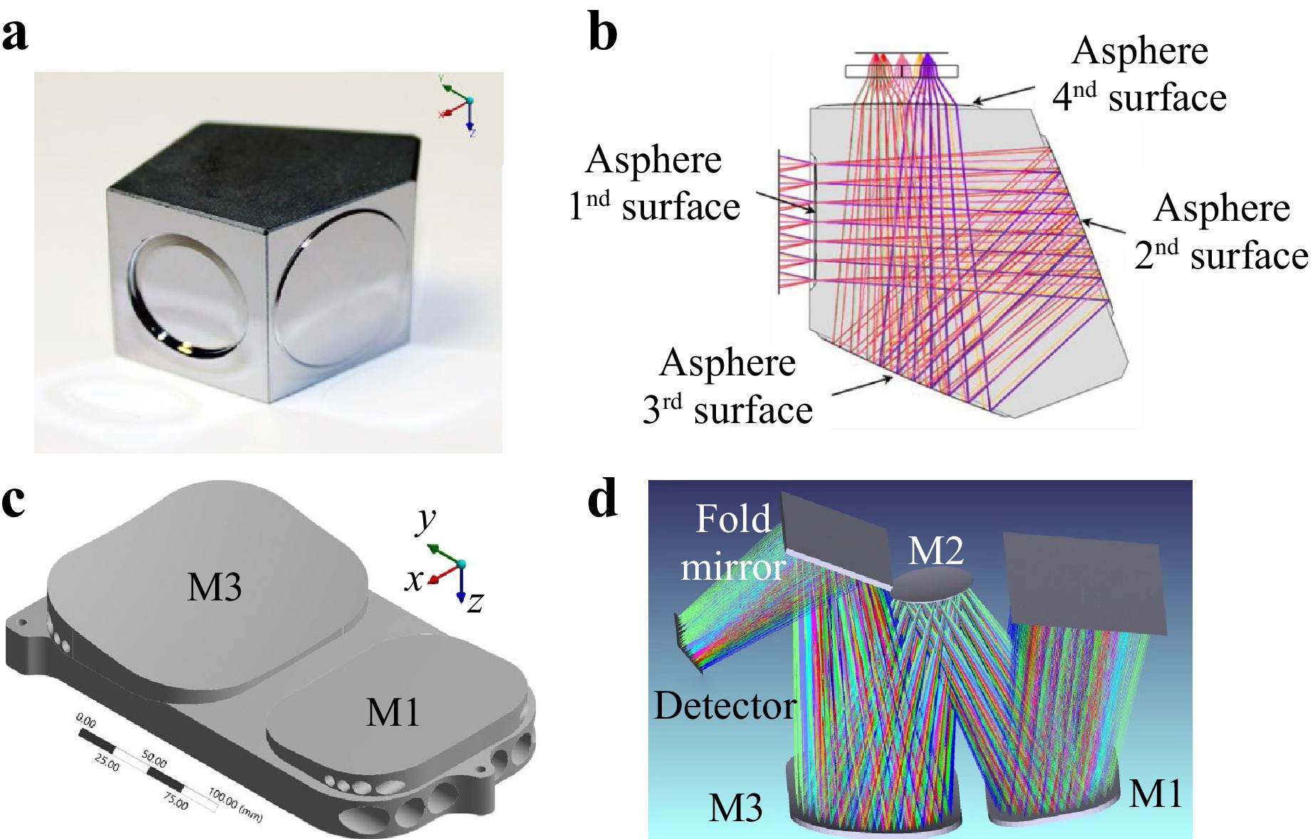
As optoelectronic performance and structural compactivity continuously improve in major equipment and advanced instruments, the demand for high-precision and integrated optical systems has become increasingly urgent in aerospace, astronomy, and industry^1–4. The traditional approach of individually fabricating, testing, assembling, and subsequently fine-tuning each element and functional surface in a cumbersome integration process with limited reliability. In recent years, monolithic multi-freeform optical structures have attracted intensive attention owing to their powerful capability to reduce assembly complexity while guaranteeing functionalities during the whole service period^5–7, as shown in Fig. 1. However, both the surface forms and their relative positions determine the functionality of the optoelectronic system. Therefore, measuring a structured element poses significant challenges due to its complex surface form, stringent precision requirements, high dynamic range, variable relative positions among functional surfaces, and the difficulty in establishing a consistent datum system.

Fig. 1  Instances of monolithic multi-freeform optical structures. a Monolithic element and b corresponding optical design⁶. c M1 and M3 conformal optical element and d corresponding optical design⁷.

Currently, there are few mature systems capable of measuring and characterising multiple surfaces of a structured element at one stop⁸. A coordinate measuring machine (CMM)⁹ is competent; however, it can only achieve micrometre-level precision, and point-wise contact measurements may damage the workpiece. Therefore, some researchers conducted rough measurements using a CMM and subsequently conducted fine measurement using deflectometry or profilometry after corrective machining¹⁰. However, this approach is inefficient. Other researchers have enhanced the measurement efficiency by replacing the contact probes with noncontact sensor⁸. Interferometry using computer-generated holograms (CGHs) has attracted considerable interest in measuring freeform structures^11–12. Auxiliary retro reflectors and alignment holograms are fabricated outside the diffraction null on the substrate, enabling collaborative form-position measurement by aligning the CGH, interferometer, and reference datums on the workpiece^13–14. These methods incur higher costs^15–16 and the design and fabrication of the workpiece reference and CGHs must be synchronised. Additionally, it is challenging to accommodate multiple surfaces with salient positional differences within one interferogram owing to the limited measurement range of interferometry. Some researchers have attempted to design and fabricate global references for all functional surfaces⁶, but the complexity of those fabrication and measurement procedures hinders practical application. Other researchers conducted point-scanning measurements using a chromatic confocal sensor (CCS) mounted on a high-precision multi-axis system¹⁷. However, this approach is costly and inflexible. Overall, the measurement of a structured element remains highly complex and costly. It is urgent to develop simultaneous form-position measurement approaches for multiple functional surfaces.

Phase measuring deflectometry (PMD) is a powerful technology^18–20, particularly suited for complex optics owing to its simple structure, low cost, superior flexibility, and broad dynamic range²¹. However, despite its exceptional sensitivity to surface gradients, PMD exhibits low sensitivity to the position of the surface under test (SUT)²⁰. Consequently, traditional PMD often ignores piston, tip, and tilt terms derived from the measured form²². However, this hampers its applicability for simultaneous form-position measurements. The error arises mainly at two stages, namely the geometric calibration and workpiece positioning. On one hand, accurate geometric calibration is challenging. The predominant approaches are machine vision-based methods with the aid of reflecting mirrors, such as plane mirrors with or without markers^23–24, stepped mirrors²⁵, and spherical mirrors²⁶, as the camera cannot directly observe the screen. Although these methods endeavour to achieve full-rank calculations to determine the geometric configuration parameters of the system, degeneracy issues frequently arise in practice²⁷. The contributing factors include insufficient markers, singularity resulting from the position configuration, limited curvature of spherical mirror. Moreover, the optimisation curve may become excessively smooth because of coupling relationship between the different configuration parameters. The optimisation process can be trapped at local optima, resulting in significant calibration errors. On the other hand, workpiece positioning presents a classic challenge due to the inherent slope-height ambiguity²² issue lying in monoscopic deflectometry. The primary approaches to addressing this issue involve introducing appropriate regularisation constraints, which encompass but are not limited to, stereovision, multiple screens, a height-given seeding point, nominal-given form etc^19–20. Unfortunately, these methods generally obtain inaccurate results for the absolute positions. Overall, the errors introduced by the system geometric calibration and workpiece positioning introduce significant low-order measurement errors in deflectometry. Other error sources, such as inaccurate camera models²⁷ and imaging aberrations²⁸, primarily contribute to high-order errors. And they will be discussed in future studies.

In this study, a simultaneous form-position measurement method based on Bayesian multi-sensor fusion is proposed. A multisensor system was constructed through an in-depth analysis of the limitations of the PMD on positioning. A CCS and rotary table were integrated into the deflectometric system to enhance the system sensitivity against the position of the SUT. The calibration and measurement processes are converted into a state estimation problem²⁹ by leveraging Bayesian theory to infer multisensor observations probabilistically. The remainder of this paper is organised as follows: The basic principles are outlined in the Methodology section. Comprehensive experimental validations are presented in the Results section. Further discussion and conclusions are presented in the Discussion and Conclusion sections, respectively.

First, a PMD system serving as the primary sensor is introduced. The measurement can be regarded as a process of specifying and integrating the surface gradients, as shown in Fig. 2a.

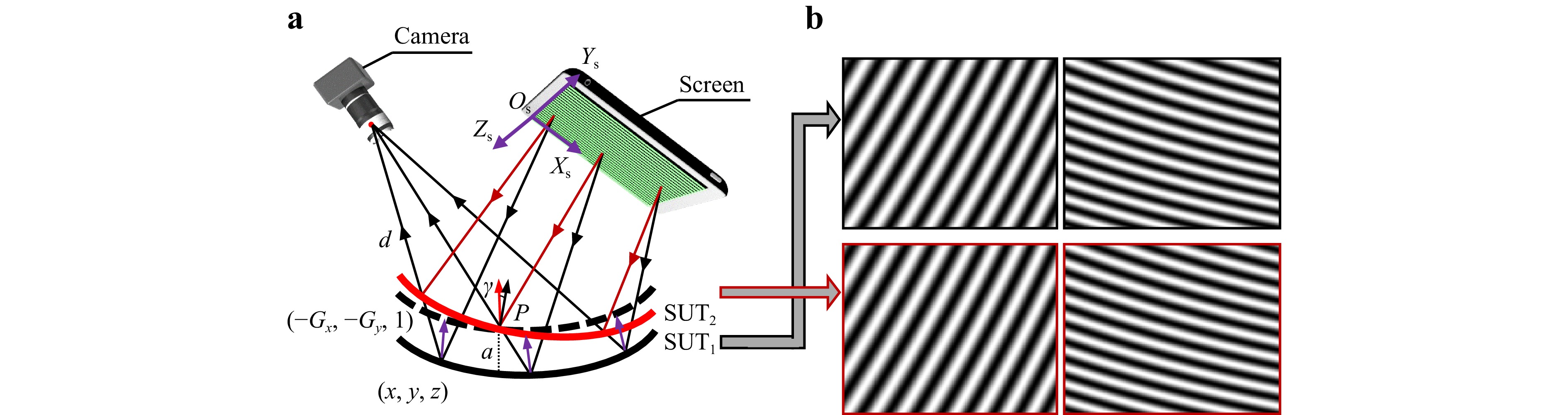
Fig. 2  Schematic diagram of PMD. a Coupling between slope and position. b Consistent observations for different combinations of forms and positions.

where intg (·) denotes the integral operation, z represents the height map of the SUT, (x, y) are the lateral coordinates of measured points, and (G_x, G_y) are the partial gradients along the x- and y-directions. Specifically, the coordinates (x, y) define the position, while (G_x, G_y) determine the orientation. The position and orientation depend on the distance d between the camera’s optical centre and the measured point, as well as the camera-screen relative pose. However, as aforementioned, existing workpiece positioning methods^19–20 cannot achieve high-precision positioning. Furthermore, those geometric calibration methods based on machine vision^23–26 are prone to local minima due to the degeneracy occurring in the numerical calculation, resulting in significant errors.

Notably, position and orientation are coupled to each other in deflectometry due to the underlying slope-height ambiguity issue²². As illustrated in Fig. 2, if shifting SUT1 by a distance a, the resulting measured result will be SUT2, which has a relative tilt angle γ concerning SUT1. These two results correspond to identical fringe images, as shown in Fig. 2b. Only a small form deviation exists between these two if the relative positional differences are eliminated by registration, which is normally 100-1000 times smaller than the positional deviation owing to the lever amplification effect of the rays³⁰. Therefore, deflectometry is not suitable for the simultaneous form-position measurement of multiple surfaces of structural elements.

Consequently, it is crucial to eliminate the errors introduced by inaccurate geometric calibration and workpiece positioning. A multisensor measurement system comprising a PMD system, a CCS, and a rotary table was constructed, as shown in Fig. 3. The CCS, which is used as a distance sensor, is integrated into the measurement system to provide a rigid constraint to the tracing-ray model. It enhances the accuracy of the absolute distance d from the camera to the workpiece. Furthermore, CCS provides a regularisation term for ray propagation, which mitigates the inaccuracies arising from degeneracy in the system geometric calibration solver. A rotary table was used to facilitate the measurement of different surfaces of the structure. And a positioning system combined with the CCS was established. A global coordinate system was defined on the rotary table, which resulted in virtual CCSs being used to represent the CCS at equivalent measurement positions, as illustrated in Fig. 3b. Moreover, the rotary table can also impose rigid position constraints on the relative positions between multiple functional surfaces²¹.

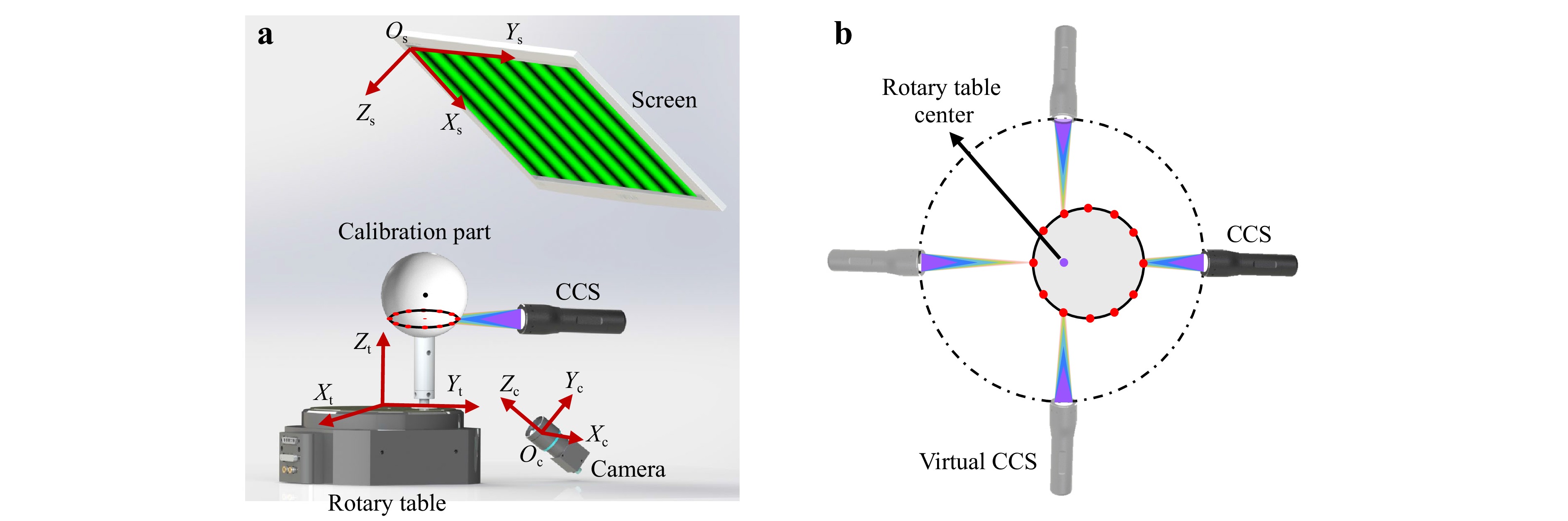
Fig. 3  Schematic diagram of the multi-sensor measurement system. a System configuration, b CCS positioning system.

From the point of view of probability, each sensor has a certain measurement uncertainty. By integrating various sources of uncertainty, the overall confidence is enhanced, which behaves as a classical filter such as the Kalman filter²⁹. The stronger the complementarity between the sensors, the higher the information utilisation rate. The PMD system has high uncertainty in specifying the absolute position but low uncertainty in measuring the normal directions of the SUT, whereas the CCS has the opposite characteristics. Therefore, combining them can effectively enhance the form-position measurement precision.

System calibration is implemented to encompass the intrinsic parameters and external geometric parameters of the individual sensors and ensure the collaborative functionality of the multisensor. For the calibration of intrinsic parameters, the camera can be readily calibrated using well-established techniques³¹, and the specifications of a commercial CCS are typically provided by suppliers. Geometric calibration plays a dominant role for the measurement accuracy. For clarity, certain notations are defined. The coordinate frames of the camera, screen, CCS, spherical standard, and rotary table are denoted by {c}, {s}, {l}, {p}, and {t}, respectively. In the study, {t} is defined as the global coordinate system. The rotation matrix, the Euler angles and the translation vector are represented by R, θ and T, respectively. For example, R_c represents the rotation matrix from camera coordinate system {c} to global coordinate system {t}.

Geometric parameters are typically calibrated by constructing a proper solver in conjunction with a known reference feature. Specifically, geometric calibration can be implemented by rotating a spherical standard through one full revolution on a rotary table, recording multi-sensor observations at several positions with an angular interval of α. The camera captured a sequence of distorted fringe images reflected by a sphere. Under the co-planarity constraint^32–33, the relationship between {c}, {s}, and {p} can be uniquely determined by bundle adjustment, indicating that the sphere centre lies on the plane formed by the incident and reflected rays. In addition, {t} can be unified by fitting the positions of spherical standard. In addition, CCS can specify the relative positions of {l}, {p}, and {t}. Specifically, the translation vector of the CCS T_l and that of the spherical standard T_p can be determined when the CCS direction n_l is known, as described in Eq. (2). Furthermore, n_l can be calibrated using a machine-vision-based method or CMM.

with $ {\boldsymbol P} = {{\boldsymbol T}_l} + v{{\boldsymbol n}_l},\beta = f\left( {\boldsymbol P} \right) - T_p^{\textit z} $

where r₀ is the radius of the sphere standard and T^x, T^y and T^z represent the x-, y-, and z- components of the translation vector, respectively. v denotes the distance along n_l between the CCS and the measured point, and P denotes the points measured by the CCS in the coordinate system {t}. f(·) represents the circle fitting function and outputs the z-component of the circle centre. Loss(·) is a linear rectification function used to formulate a regularization term that discriminates whether the CCS is positioned above or below the sphere standard. With {p} serving as a bridge, the geometric parameters can be collaboratively obtained by the two sensors within a common coordinate system. Notably, the position constraints of the spherical standard along the x- and y-directions are provided by both CCS and PMD, while that in the z-direction is solely from the PMD system. This is because the absolute z-component of T_l and T_p cannot be uniquely determined by the CCS, even when their relative positions are provided.

The calibration solver was converted into a state-estimation problem. The geometric configuration parameters s = {T_p, T_l, θ_c, T_c, θ_s, T_s} can be calculated by the Bayesian inference³⁴. The Bayesian theorem is employed to estimate the conditional distribution of s.

where O_F and O_L denote the observations from the PMD and CCS systems, P (s |O_F, O_L), P (O_F, O_L |s), and P (s) denote the posterior, likelihood, and prior probabilities, respectively. P (O_F, O_L) denotes the normalising constant, which is omitted for simplicity. Directly calculating the posterior probability is extremely challenging, and normally, priors cannot be obtained before system calibration. Consequently, the solver can be converted to maximise the likelihood probability as follows:

Moreover, assuming the measurement noise follows a Gaussian distribution, the likelihood probability can be denoted as

where μ(s) is the expectation of s, and $ \boldsymbol\varSigma $ denotes the covariance matrix of the sensor observations. When considering a single observation, minimising the negative logarithm can be leveraged to calculate the maximum likelihood estimate owing to the favourable properties of the Gaussian distribution. This can be converted into a least-squares solver because the observations and inputs are mutually independent, namely

where h (·) and g (·) represent the observation models for the PMD and CCS systems, respectively, and e_F and e_L denote observation residuals from PMD and CCS, respectively. $ \boldsymbol\varSigma _{\text{F}}^{ - 1} $ and $ \boldsymbol\varSigma _L^{ - 1} $ denote the information matrices; specifically, the inverses of the covariance matrices. A flowchart of the system calibration is shown in Fig. 4.

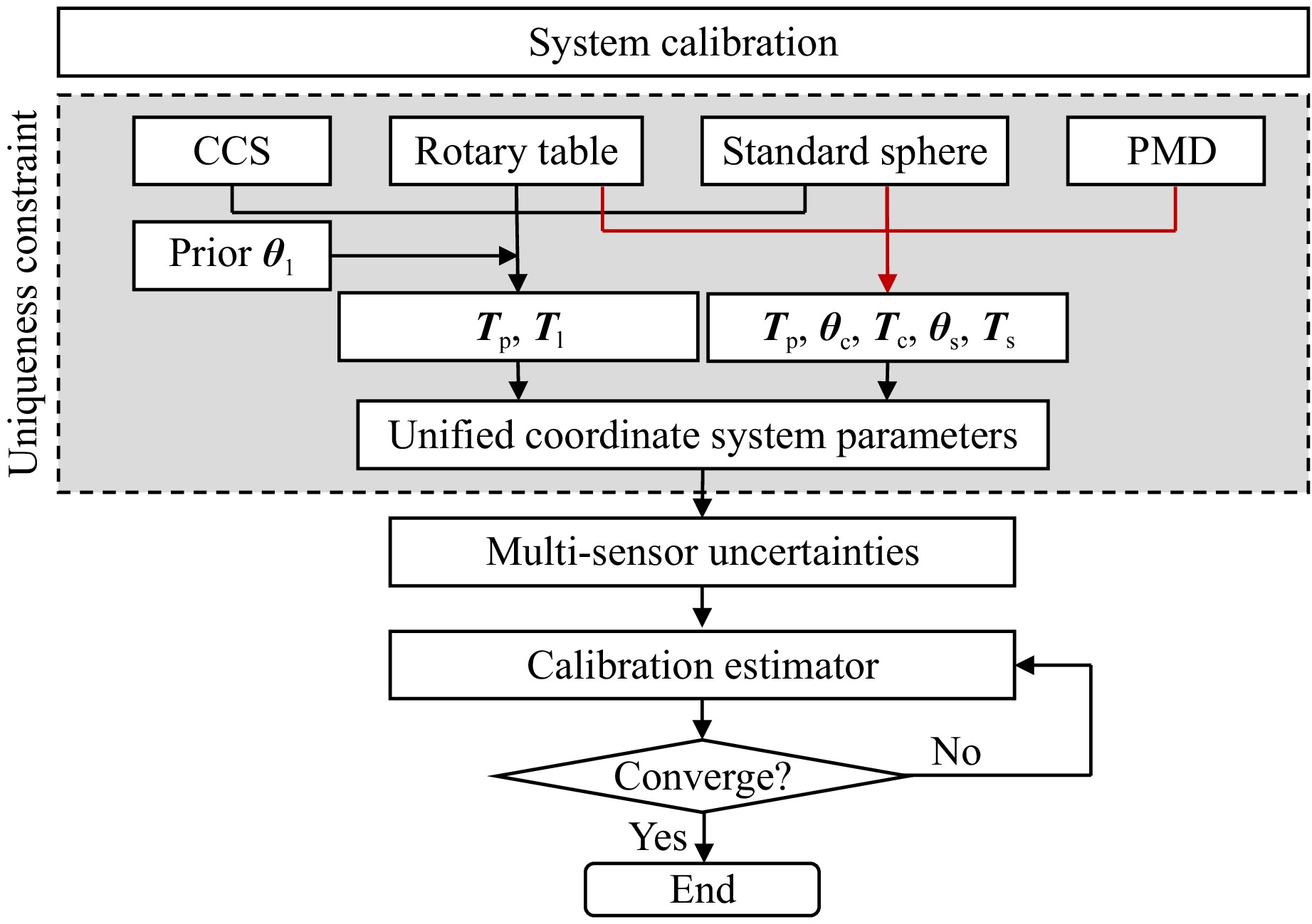
Fig. 4  Flowchart of system calibration.

The calibration solver was reformulated as a least-squares optimisation problem, in which the effort was mainly focused on calculating the information matrices. Information matrices were adopted to estimate the measurement uncertainty. The uncertainty of PMD mainly originates from the camera noise³⁵,

where $\sigma_I^2 $ denotes the variance of the image intensity I captured by a camera, K denotes the overall gain, I_dark denotes the dark current, $\sigma_d^2 $ denotes the variance of all the noise related to the sensor readout and amplifier circuits. Moreover, $\sigma^2_q $ = 1/12 (DN²) denotes the quantisation error³⁵.

Subsequently, a comprehensive error-propagation chain is established, as shown in Fig. 5. Specifically, the intensity noise is propagated to the phase distribution through encoding and decoding operations, which, in turn, affects the correspondence between the camera and screen pixels. The correctness of the correspondences directly affects the measurement accuracy of the PMD; hence, the re-projection error is used to quantify the measurement uncertainty. The Monte Carlo method³⁶ was employed to model error propagation.

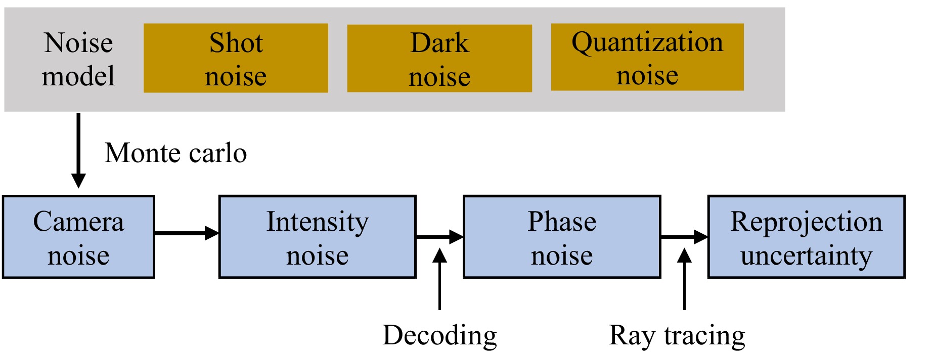
Fig. 5  Uncertainty estimation of PMD.

The form and position parameters were obtained simultaneously based on multisensor observations, which is a process analogous to system calibration. Each surface of the freeform structure was measured at an appropriate angular position of the rotary table. A two-step estimation method is proposed to achieve a more accurate result. First, a low-order position estimator is adopted to provide a reliable initial value. Second, a form-position estimator refines all low-mid-high-order components of the surface.

To mitigate the impact of calibration errors on measurement results, conventional approaches adjust the configuration parameters using the measurement results¹⁹. The solved parameters are considered correct when the resulting measured form associated with the current configuration matches the nominal form of the SUT. However, such an assumption is not always reasonable, that is, a false convergence of the configuration parameters may occur because of the asymmetric form error, complex surface form, and ill-conditioning of the numerical optimisation problem. Therefore, a holistic positioning method was devised to guarantee the reliability of the positioning result, as shown in Eq. 8. The configuration parameters and positions of all the functional surfaces of the system were solved concurrently within a global optimisation framework. In addition, it incorporates a calibration module with uniqueness constraints, as illustrated in the System Calibration section.

where m denote the positional parameters of the SUT, and λ(·) is the regularisation term. At this stage, multiple surfaces can be positioned and the configuration parameters are updated accordingly.

Subsequently, another estimator was constructed for form reconstruction. The form-position data can be represented using a linear combination of mathematical expressions, such as Zernike polynomials and B-splines etc.,

where w is the coefficient vector of the mathematical expressions. It is important to note that the information matrices $ {\boldsymbol\varSigma '}_{\rm F}^{ - 1} $ and $ {\boldsymbol\varSigma '}_{\rm L}^{ - 1} $ must be recalculated for tightly coupled sensor values. Both the inherent uncertainty of the sensor and the geometric uncertainty resulting from the calibration must be considered simultaneously. The uncertainty of configuration parameters can be determined by certainty propagation theory³⁷:

where σ² denotes the variance, J represents the Jacobian matrix associated with the configuration parameters, and W denotes the reciprocal of the squared observation residuals, which is a sparse matrix. Uncertainty modelling through the Monte Carlo method is similar to that detailed in the Uncertainty Estimation, with the only difference being the incorporation of geometric uncertainties into the measurement model through ray tracing. The revised information matrix ${ \boldsymbol\varSigma }' $ estimation marginalises the calibration priors in the measurement process, thereby effectively constraining the measurement results. This avoids the overfitting issue arise in the traditional modal PMD¹⁹. Ultimately, the form-position solution can be obtained via the optimisation process outlined in Eq. 9 and subsequently substitute the coefficients w into the mathematical expressions, as shown in Fig. 6.

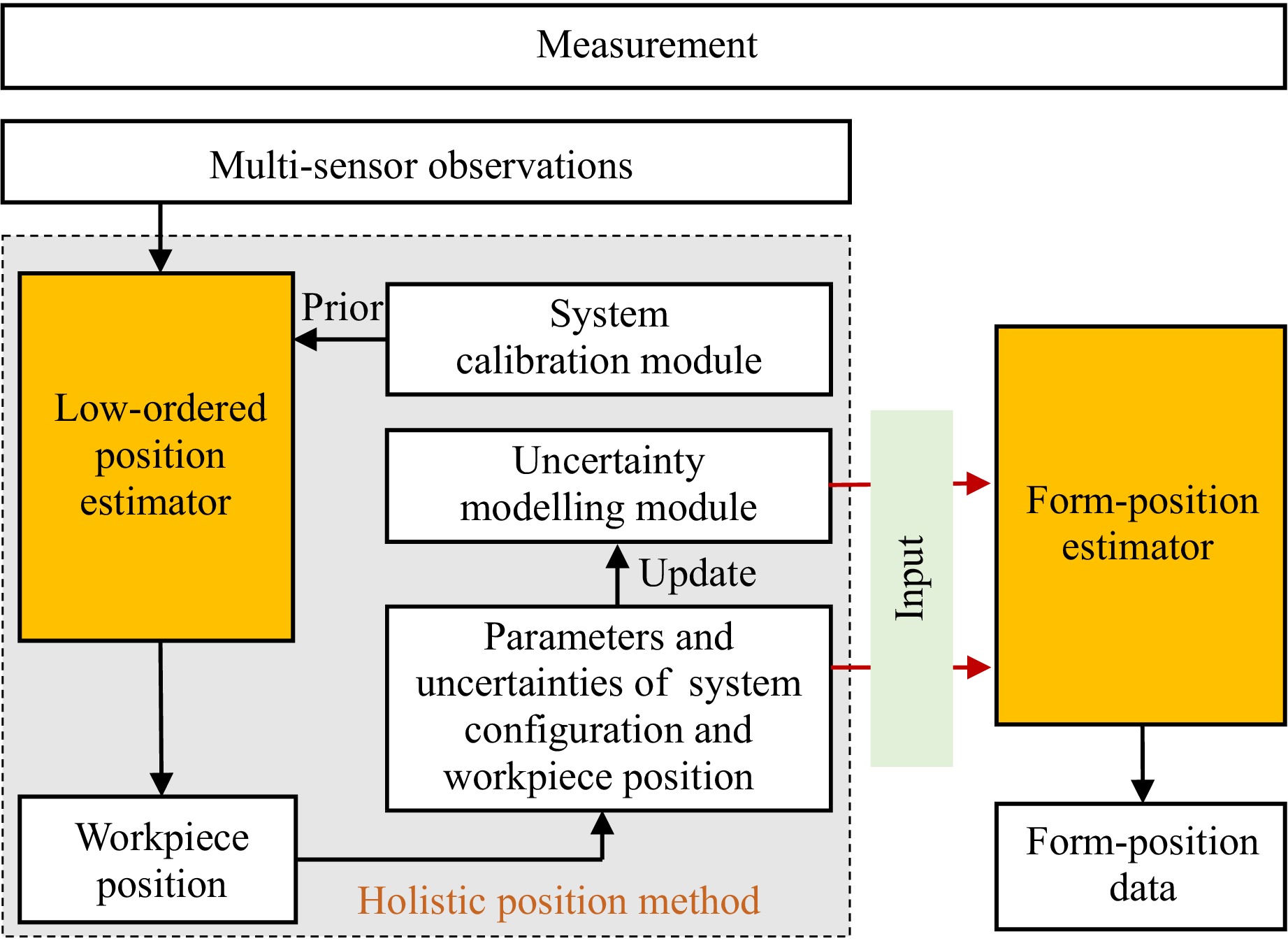
Fig. 6  Flowchart of the measurement.

There is a lack of well-acknowledged specifications for assessing the form-position quality of freeform structures⁸. A stepwise approach to assess the form and position quality of the structured element. Form assessment was conducted by registering the measured point clouds with a reference dataset obtained from third-party instruments, using the root-mean-square (RMS) and peak-to-valley (PV) of the relative residuals as metrics. For position assessment, a geometric-constraint-based iterative closest point method was developed. Specifically, the point clouds of multiple surfaces measured by a CMM were taken as a reference for position assessment and registered with the measured result.

where (R, T) denotes the optimal registration pose, and (X_CMM, Y_CMM, Z_CMM) and (X_M, Y_M, Z_M) denote the CMM data points before and after transformation, respectively. w represents the coefficients of the mathematical function. k(·) represents the z- component of the registration residuals between the CMM and constructed surface at (X_M, Y_M). Two metrics, the PV and the mean of the registration residuals, were defined to assess the positioning error according to International Geometrical Product Specifications (GPS) standards³⁸. Specifically, the point set is moved as a whole during registration, keeping the relative positions between multiple functional surfaces unchanged. This implies that all the surfaces share the same motion parameters. The underlying geometric constraints between multiple surfaces can effectively prevent mismatches caused by ambiguous features of individual surfaces. In addition, registering the point clouds with mathematical functions reduces the dependency on the sampling density and minimises the potential damage to the SUT. The framework of the proposed method is illustrated in Fig. 7.

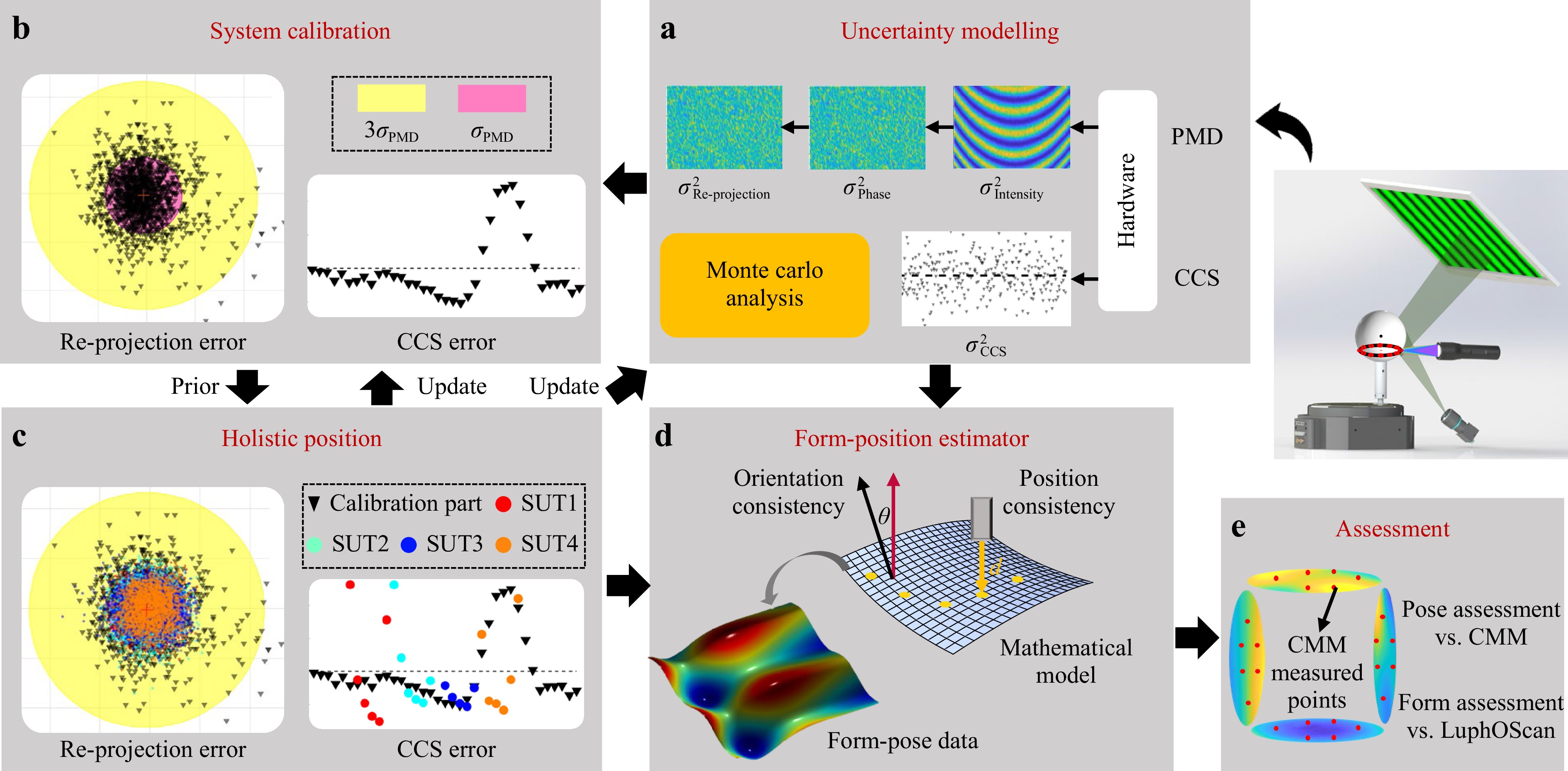
Fig. 7  Workflow of the proposed method. a Uncertainty modelling was employed to guide b system calibration and c workpiece positioning. The measurement uncertainty is updated to marginalise the relevant information into the form-position estimator d. The measurement result is compared with that of a third-party instrument e.

To verify the performance of the proposed method, a multisensor measurement system was established. The system consists of a computer monitor (AOC U28G2U with 3840 × 2160 pixels and a pixel size of 160 μm) and a CMOS camera (Basler acA1920-150 um with 1920 × 1200 pixels and a pixel size of 4.8 μm), paired with a lens of 16 mm focal length. The system also includes a CCS sensor (HongChuan C10000 with a measurement range of ±5 mm, an angular measurement range of ±13° and linear error less than ±2 um) and a rotary table (Aerotech ABRS-200 MP with a resolution of 0.079 arc sec, synchronous axial error less than 100 nm, and synchronous radial error less than 250 nm), as shown in Fig. 8.

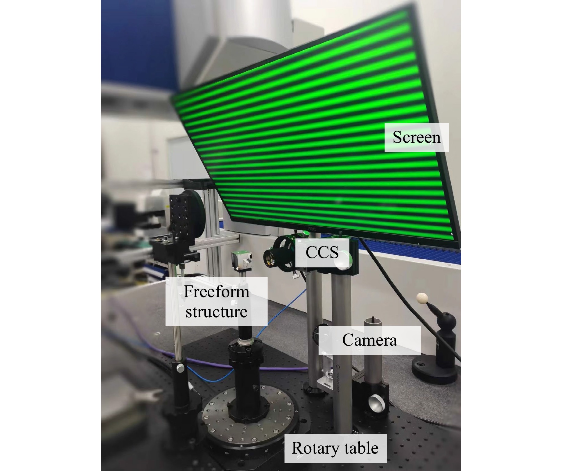
Fig. 8  Setup of the multi-sensor measuring system.

This section focuses on estimating the PMD uncertainty, while the uncertainties of other commercial sensors are provided by the suppliers. A virtual PMD system was constructed based on the actual experimental setup and pre-calibration²³, as depicted in Fig. 9a. It includes parameters such as the fringe width, contrast, codec mode, and geometric configuration³⁹. Specifically, four-step phase-shifted fringes with a period of 36 pixels were displayed on the screen. And the fringe contrast associated with the camera was set to 0.8. The camera noise parameters can be easily obtained from the camera supplier as they adhere to the European Machine Vision Association (EMVA) Standard 1288⁴⁰, as shown in Table 1. Note that the relationship between the gain and corresponding grayscale values was provided by the suppliers³⁵. The image intensity and noise distributions are shown in Fig. 9b, e, respectively. It was observed that the noise amplitude was directly proportional to the intensity. Furthermore, according to the error propagation chain established above, the intensity deviation is transferred to phase errors via a four-step phase-shifting algorithm³⁵, as shown in Fig. 9c, f, which in turn affects the correspondence between the camera and screen pixels, as shown in Fig. 9d, g.

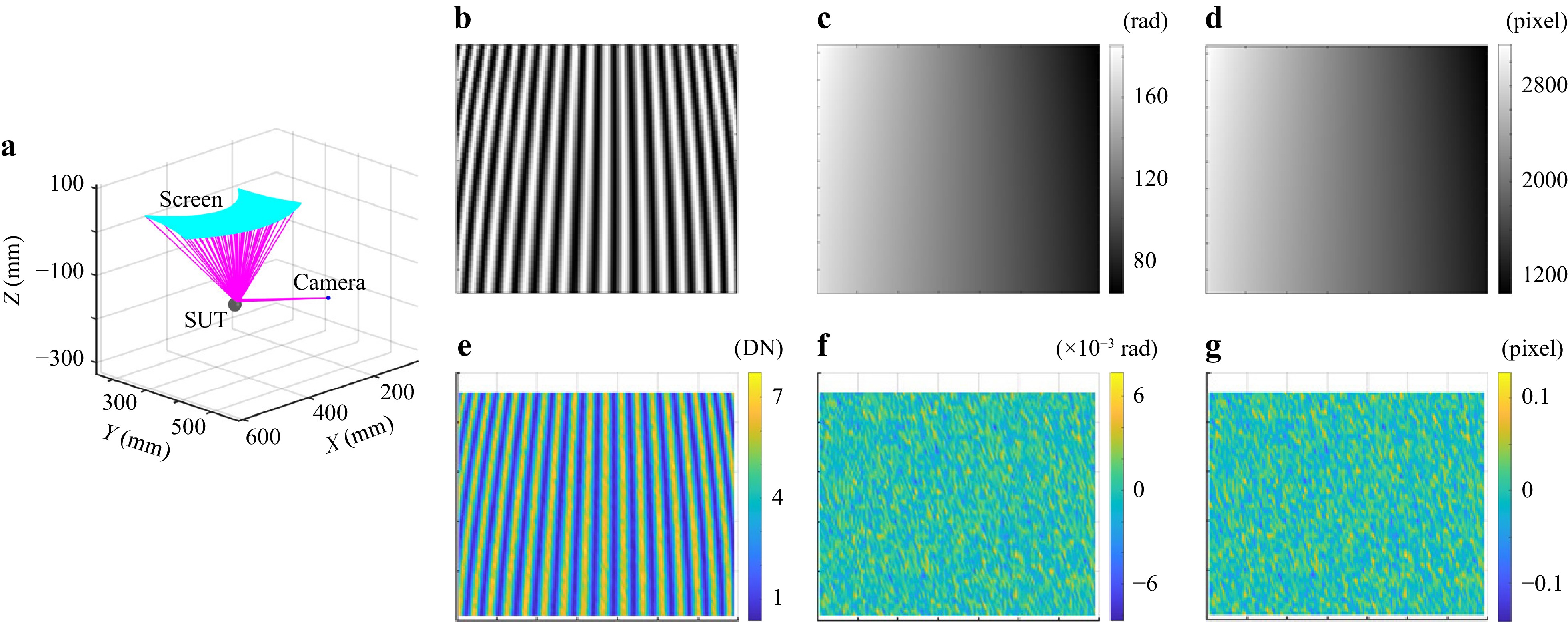
Fig. 9  The diagram of uncertainty modelling of PMD. a system configuration, b intensity, c phase, and d traced pixels of the screen, and their noise distributions e-g.

Because the calibration and measurement framework based on Bayesian inference assumes a Gaussian noise distribution for multisensor observations, it is imperative to verify whether the observations follow such a distribution. The Monte Carlo simulation was performed 1000 times. The conformation of the Gaussian distribution, as observed in the above simulations, is verified using the Jarque-Bera test⁴¹. A standard deviation of 0.0483 pixels was adopted to assess PMD uncertainty.

Notably, the uncertainty of CCS may exceed the supplier-provided values in practice. This discrepancy arises when the probe is not precisely perpendicular the SUT. These errors can be mitigated by using prior knowledge and testing. A spherical standard was used to test the CCS with the measurement uncertainty represented by the residuals from Eq. 2, instead of the parameters provided by the supplier. The air-bearing rotary table was assumed ideal because its uncertainty was extremely small.

A freeform structure was machined to verify the accuracy of the proposed measurement method, as shown in Fig. 10. It contains four optical surfaces, namely, two spherical and two aspheric surfaces, which can be uniformly expressed as

Fig. 10  Freeform structure.

where r denotes the radial coordinate, c denotes the base curvature, and K denotes a conic factor. The other higher-order coefficients are listed in Table 2.

A spherical standard with a radius of curvature of 15 mm is used for system calibration. Subsequently, the structure was rotated using a rotary table and each side surface was measured six times using a multisensor system at 5-degree intervals. The number of measurements and angular intervals can be adjusted based on the measurement range. These settings can be obtained from simulation experiments³³. The four functional surfaces of the element were positioned and reconstructed using the proposed method, as shown in Fig. 11. The two spherical surfaces R300 and R1000 were also measured using an interferometer (GPI XP/D, Zygo), while the two aspheric surfaces S1 and S2 were measured using a LUPHOScan profilometer (420SD, Taylor Hobson). A CMM (Prismo Ultra, Carl Zeiss) was used to assess the positioning accuracy.

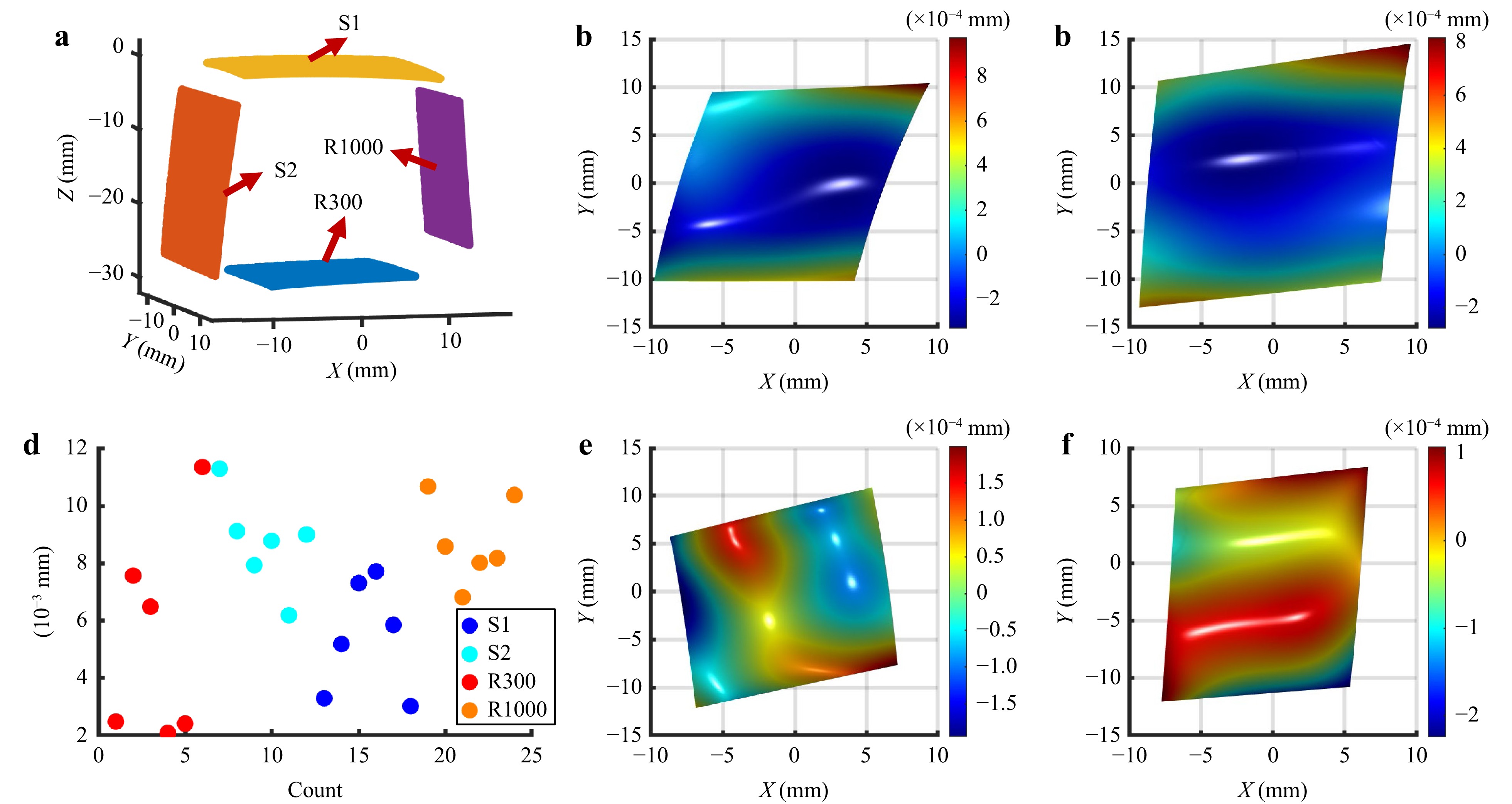
Fig. 11  Experimental results of the freeform structured element. a The measured form-position results. Form deviations of S1 b, S2 c, R300 e and S1000 f, respectively. The measured position deviations d.

The measured form-position deviations are presented in Table 3. It can be seen that the RMS of form can achieve a level of one hundred nanometres, while ten micrometres for position.

The concept of multisensor fusion leverages the complementary strengths of different sensors to fulfil the requirements of complete form-position measurement. Several aspects of the proposed method are further discussed for a comprehensive understanding.

The proposed method converts the calibration and measurement problems into state estimation problems. Furthermore, Bayesian inference was converted into a graph optimisation solver. The measurement accuracy is limited to some extent by the accuracy of the uncertainty modelling. Therefore, more accurate modelling and estimations of sensor uncertainties are required.

Holistic positioning shortens the error propagation chain and mitigates inconsistencies in geometric positional parameters across surfaces. However, holistic positioning was performed using the nominal form of the surfaces under test, and it was assumed that the positioning errors caused by form errors could be omitted. Significant positioning errors occurred when large or asymmetric form errors were present. In this case, an alternative method can enhance calibration precision by incorporating the actual positions and forms of the calibration standards while maintaining the overall applicability of the proposed method.

The fabrication accuracy of optical elements and calibration standards is sufficiently high. Therefore, holistic positioning demonstrates a certain degree of adaptability in practice because form errors are often irregular and statistically symmetric⁴². Additionally, embedding calibration module priors and multisensor constraints in the position estimator further reduces the influence of form errors.

The form-position calculation is formulated as an optimisation problem, which inevitably transmits noise from the environment or sensors to the surface. Reconstruction performance depends on the choice of mathematical models. Locally defined basis functions, such as B-splines⁴³, can outperform globally defined functions by limiting error propagation. However, these methods can be computationally intensive. Consequently, selecting reconstruction functions requires balancing measurement accuracy and computational efficiency in practical scenarios.

Manufacturing freeform structures is expensive and inefficient because the workpiece undergoes remounting and alignment between the machining and measurement equipment. The proposed method can be applied to in-situ measurements, as shown in Fig. 12. The PMD and CCS systems were mounted onto the air-bearing spindle on a single-point diamond-turning machine. It is noteworthy that the absolute positioning ability of the proposed method was limited to a certain extent owing to the restricted motion degrees of freedom. This limitation reduces the number of measurement points and introduces drift to the measurement results of the CCS, both of which adversely affect the measurement accuracy. More movement degrees of freedom and coordinate constraints can be provided by machine tool, thereby leading to higher measurement precision.

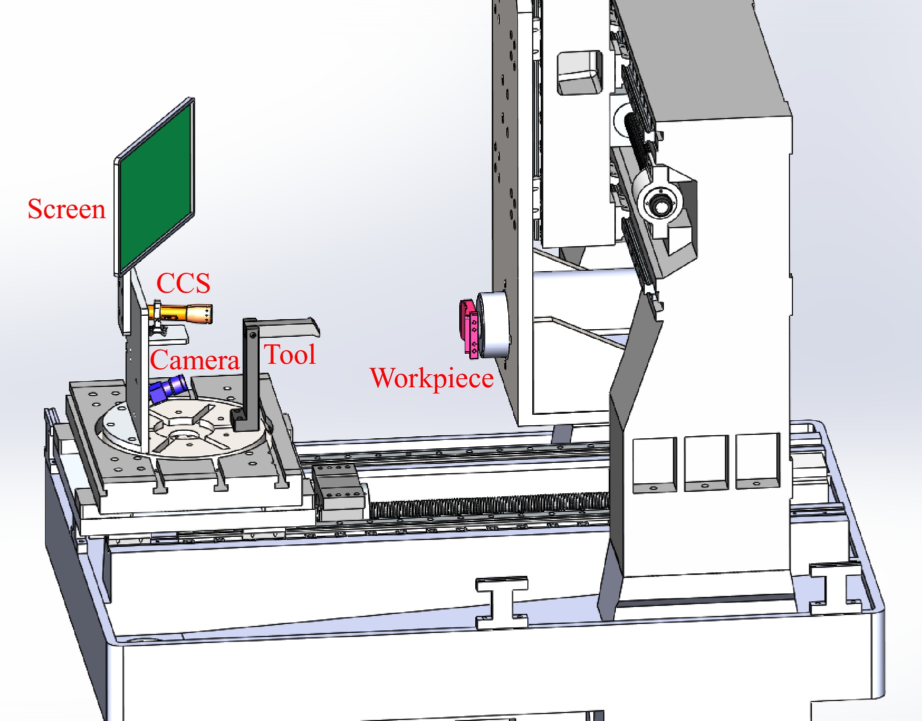
Fig. 12  Integrated in-situ measurement system mounted on the single-point diamond turning machine.

To achieve simultaneous form-position measurements for monolithic multi-freeform optical structures, a multisensor measurement system was constructed. Measurement is regarded as a reduction process of the system information entropy, thereby decreasing the prediction uncertainty through the fusion of multi-source observations. This method overcomes the positioning limitations of deflectometry and successfully elevates deflectometry from relative to absolute measurements. A measurement framework with probabilistic description capability was proposed based on physical uncertainty modelling. This infers the measurement results from an inverse problem based on physical reality, thereby addressing the statistical bias in traditional numerical optimisation. Marginalising calibration data into the measurement probabilistic framework not only effectively prevents error propagation but also enhances the utilisation of the provided constraints. This approach has a universal applicability, allowing flexible system configurations in various scenarios and fields.

This study was supported by the National Natural Science Foundation of China (52475551), the Natural Science Foundation of Shanghai (24ZR1406800), and the Dreams Foundation of Jianghuai Advanced Technology Center (2023-ZM01C008).