


-
Laser interferometry has the advantages of broad range, high resolution and good traceability. It is widely used in machine lithography, high-end equipment manufacturing, basic physics research and other fields, becoming one of the most important precision displacement measurement technologies1,2. However, the traditional laser interferometers have several shortcomings, including large size, susceptibility to thermal noise and many mechanical drifts, and difficulty to conduct measurements in narrow spaces such as inside high-end equipment3,4. Therefore, a new generation of interferometric measurement methods using microsensor heads has become a popular focus of research to realize embedded measurement in narrow spaces5. At the same time, this also brings new technical challenges.
The measurement and demodulation methods adopted in fiber microprobe sensor (FMS) include white light interferometry6,7, orthogonal point intensity detection8 and phase generated carrier (PGC) demodulation method. The last one has become the most important method for dynamic displacement measurement adopted in FMSs because of its advantages of superior dynamic characteristics and sensitivity9–15. Laser interferometry based on PGC usually adopts two light source modulation methods: external modulation and internal modulation. External modulation is typically achieved by attaching an acousto-optical or electro-optical modulator to the optical path, which, however, produces the sensing structure too large to be used in microprobes9,10. Internal modulation is generally obtained by directly changing the laser characteristics by varying the injection current. Therefore, the method does not require additional devices and is suitable for microprobe sensing11–13. However, in the PGC demodulation based on internal modulation, incorrect phase modulation depth (PMD) can lead to large periodic nonlinear errors, which severely restricts the displacement measurement accuracy. Researchers tried to correct nonlinear errors present in the results. Yan14 used four pairs of quadrature harmonic components to eliminate the effects of PMD, but the method required four times as much hardware processing resources as the traditional method. Another approach to correcting the errors caused by PMD is the ellipse fitting algorithm15, which need offline processing and more calculations. In summary, due to the lack of a model for light source modulation parameters and measurement characteristics in PGC demodulation based on internal modulation, measurement errors can only be corrected in the results but cannot be eliminated at the source, which complicates the algorithms and causes residual error.
On the one hand, the laser carried out high-bandwidth and large-amplitude frequency modulation to realize high-speed and high-precision measurement in the FMS, as explained in the following sections. On the other hand, as the measuring scale of FMS, the laser center wavelength has to be stabilized under above modulation to achieve high measurement stability.
To achieve the laser center wavelength stabilization, the standard F-P cavity and gas molecular absorption spectral line are often used as the external reference. Compared to the F-P cavity16, the molecular absorption frequency stabilization method is widely used because of its simple structure and better integration and stability of commercial gas chambers. Several in-depth studies17,18 have been conducted on the external cavity diode laser (ECDL) frequency stabilization technology adopting absorption gas chambers, but due to the structural characteristics of ECDL, its modulation amplitude and frequency are small and slow, respectively. Furthermore, the ECDLs are not suitable for commercial FMS due to their high cost. In contrast, because of the advantages of small size and good tuning performance19, the distributed feedback (DFB) laser was widely used to perform frequency stabilization based on the saturated absorption gas chamber to realize the FMS precise measurements20,21. However, in these studies, the modulation frequency was below 10 kHz and the modulation amplitude was small, which can lead to a poor measurement performance. Aketagawa et al. improved the laser wavelength modulation frequency to 300 kHz, but the modulation amplitude of 25 MHz was still insufficient for embedded measurement of small distance22. Klaus et al. raised the modulation frequency to the MHz level, but the impact of high-bandwidth and large-amplitude frequency modulation on the frequency stabilization system was ignored, which can cause the system off-lock23. From the above literature review, it can be seen that the existing frequency stabilization methods and models are only applicable to the low-bandwidth and small-amplitude frequency modulation. Moreover, laser center wavelength of the FMS cannot be stabilized or locked when the laser carries out high-bandwidth and large-amplitude frequency modulation, which results in inaccurate interferometer measurements and unreliable measurement stability.
In this article, a complete model of the light source characteristics and measurement accuracy of high precision fiber microprobe sensor based on PGC demodulation are presented. High-bandwidth and large-amplitude frequency modulation is used to address the nonlinear measurement error at the source of the PGC algorithm. The opposing mechanisms of wavelength modulation and central frequency stabilization are revealed and analyzed for the first time along the measurement distortion. A modified frequency stabilization model and method for the laser light source under high-bandwidth and large-amplitude frequency modulation is proposed, which improves the measurement accuracy to enable sub-nanometer measurements.
The remaining sections of this paper are arranged as follows: in the second section, the complete model about light source characteristics and measurement accuracy of high precision fiber microprobe sensor based on PGC demodulation is presented. The nonlinear errors of tens of nm are analyzed and resolved. Subsequently, the opposing mechanism in the frequency stabilization system under high-bandwidth and large-amplitude frequency modulation is analyzed and a wavelength stabilization method to improve the measurement accuracy is proposed. In the third section, the experiments performed to verify the performance and efficiency of the method proposed in this paper are discussed.
-
In FMSs with laser frequency modulation, the phase of the interference signal is modulated. Under ideal conditions, the interference signal S(t)13, which encodes the measured displacement information changing with time t, is given by
$$ S(t) = {k_U}{I_0} \cdot [1 + {k_v}\cos (C\cos {\omega _0}t + \varphi (t))] $$ (1) where kU is the intensity/voltage conversion coefficient, I0 is the intensity of the detected interference signal, kv is the interference signal visibility, ω0 is the carrier angular frequency and also the laser modulation bandwidth, C is the phase modulation depth, and φ(t) consists of the initial phase and the phase shift φ caused by the measured displacement x. The carrier phase modulation depth is given as
$$ C = \frac{{4{\text π} {n_{{\text{air}}}}L\Delta {\nu _m}}}{{\text{c}}} $$ (2) where c is the speed of light in a vacuum, nair is the refractive index in air, $ \text{Δ}{{v}}_{{m}} $ is the modulation amplitude of laser wavelength (frequency), and L is the working distance (WD) of the interferometer. The relationship between φ and x is as follows:
$$ x = \frac{{\varphi \cdot \lambda }}{{4{\text π} \cdot {n_{{\text{air}}}}}} $$ (3) where λ is the laser light source wavelength. The φ value is calculated by the PGC algorithm, and then x is obtained.
For the PGC-Atan demodulation algorithm16–18, the interference signal is first multiplied by the first-harmonic carrier signal ${\cos}{\omega }_{0}t $ and the second-harmonic carrier signal ${\cos}2{\omega }_{0}t $, respectively:
$$ {u_1} = {J_1}(C)\sin (\varphi (t)) $$ (4) $$ {u_2} = {J_2}(C)\cos (\varphi (t)) $$ (5) $$ \varphi (t) = \arctan \left( {\frac{{{u_1}}}{{{u_2}}}} \right) $$ (6) where J1(C) and J2(C) are the first and second-order Bessel functions at point C, respectively. Then, two orthogonal signals u1 and u2 are low-pass filtered. Subsequently, the ratio u1/u2 is obtained and the arctangent of the ratio is calculated to obtain the target phase φ(t).
According to the demodulation principle of PGC, the PGC-Atan demodulation requires the values J1(C) and J2(C) be the same, otherwise periodic nonlinear errors of tens of nm will be generated. For more information, please refer to the first part of the Experimental validation section, where we analyze the nonlinear errors at different C values through simulations. Fig. 1a shows the changes in J1(C) and J2(C) with respect to $ {\text{Δ}}{{v}}_{{m}} $ obtained from Eq. 2 when L is 2.4 cm, 4 cm and 5.6 cm, nair is 1 and c is 3 × 10⁸. When L is 4 cm, to ensure accurate demodulation results, the first intersection point of the J1(C) and J2(C) curves is generally taken, i.e., C is 2.63, for which the corresponding $ {\text{Δ}}{{v}}_{{m}} $ is about 1.57 GHz. From Fig. 1b, it can be seen that when the modulation amplitude is around 1.57 GHz, the signal-to-noise-and-distortion ratio (SINAD) is the highest and the signal quality is the best in the observation range. As L further decreases, $ {\text{Δ}}{{v}}_{{m}} $ needs to increase. When L is 2.4 cm, $ {\text{Δ}}{{v}}_{{m}} $ needs to reach about 2.61 GHz.
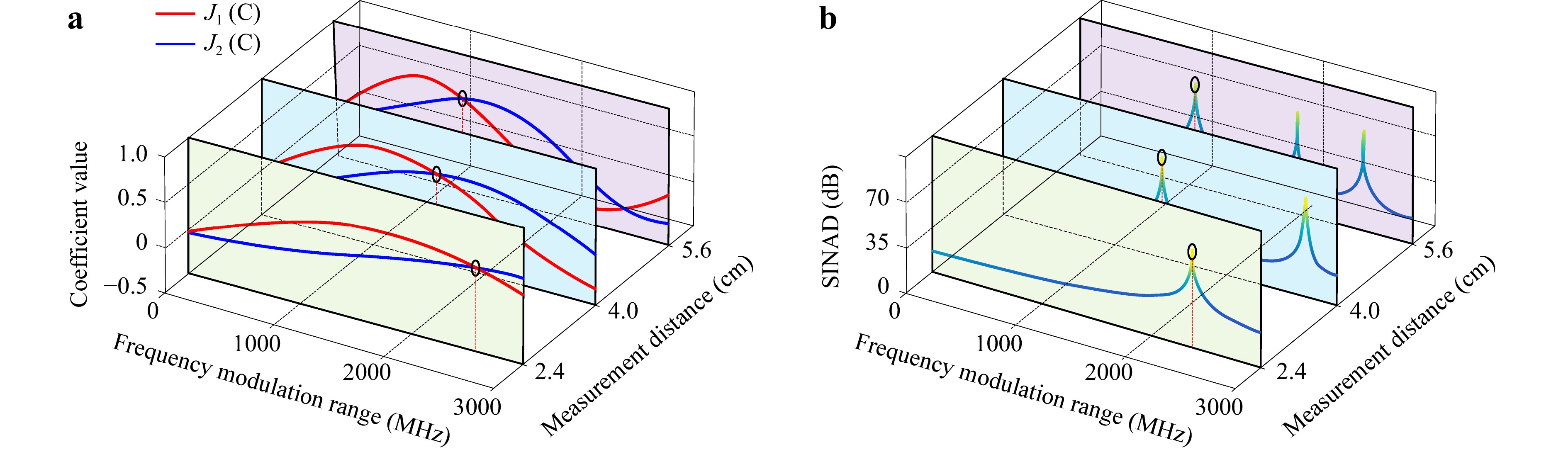
Fig. 1 Bessel functions and SINAD of FMS under different laser frequency modulation amplitudes for working distances of 2.4 cm, 4 cm and 5.6 cm.
-
Next, to explore the relationship between the upper limit of the dynamic range (i.e., the upper limit of the measurement speed) of the interference system and the laser modulation bandwidth, we simulated and carried out spectrum analysis of the interference signals obtained when the object was at rest and in uniform motion. In Fig. 2a−c, corresponding to the object at rest, the motion frequency fs = 300 kHz and the motion frequency fs = 500 kHz respectively, the red line is the upper side band of the first harmonic, and the green line is the lower side band of the second harmonic.

Fig. 2 Spectra of simulated object moving uniformly at different motion frequencies fs for laser modulation bandwidth f0 = 1 MHz. a fs = 0 Hz, b fs = 300 kHz and c fs = 500 kHz.
The relationship between the upper limit of the dynamic range of the interference system and the laser modulation bandwidth can inferred from Fig. 2:
(a) When the object was at rest, cosφ(t) was a constant. Therefore, according to Eq. 1, the spectrum of the interference signal in this case is in the form of a Fourier series with the base frequency f0 = 1 MHz. The red and green spectral lines, corresponding to the first and second harmonic components in Fig. 2a, do not exhibit spectrum shift, thus, there is no spectral aliasing between them.
(b) When the object moved at a constant speed with a motion frequency fs = 300 kHz, cosφ(t) was a cosine signal, and the spectrum of the interference signal can be regarded as a ± fs spectrum shift of each harmonic component shown in Fig. 2a. According to the principle of PGC demodulation, the prerequisite for the demodulation system to work correctly is to demodulate the first and second-harmonic signals of the interference signal without spectrum aliasing. The red line representing the upper side band of the first harmonic and the green line representing the lower side band of the second harmonic demonstrate these demodulation requirements are met.
(c) When the motion frequency increased to fs = 500 kHz, the red line and the green line just overlapped and the PGC demodulation system cannot extract the correct phase information.
In summary, it can be concluded that to increase the upper limit of the dynamic range of the interference system as much as possible without spectrum aliasing, the laser modulation bandwidth f0 and the object motion frequency fs should satisfy f0 ≥ 2fs. If the hardware conditions permit, f0 should be increased as much as possible to improve the upper limit of the dynamic range of the system, and finally f0 should be set as 1 MHz.
-
This section will further analyze the influence of the laser wavelength stability on the interferometric displacement measurements. The displacement measurement error can be calculated as follows:
$$ \begin{split} \delta L =\;& L \cdot \left( {\frac{{\delta \lambda }}{\lambda } - \frac{{\delta {n_{{\text{air}}}}}}{{{n_{{\text{air}}}}}}} \right) + \frac{\lambda }{{4{\text π} \cdot {n_{{\text{air}}}}}} \cdot \delta \varphi \\ = \;&L \cdot \left( {\frac{{\delta \lambda }}{\lambda } - \frac{{\delta {n_{{\text{air}}}}}}{{{n_{{\text{air}}}}}}} \right) + \delta {L_{idle - zone1}} + \delta {L_{idle - zone2}} + ... \end{split} $$ (7) It can be seen from Eq. 7 that the error of the measurement system can be divided into two categories. One is proportional to the measured displacement L and is called proportional error, the other is independent of the measured displacement and is called non-proportional error. The non-proportional error comprises several parts: the instrument idle zone error, instrument cosine error, instrument nonlinear error and others. For the non-proportional error, we focus on the idle zone error. This part is further sub-divided into two parts. The first one, $ {\delta L}_{idle-zone1} $, is caused by the effect of wavelength jitter on the idle area, and the other, $ {\delta L}_{idle-zone2} $, is caused by the change in environmental refractive index.
In this paper, we focus on analyzing the effect of proportional error (Eq. 7) on measurement accuracy. The accuracy of the refractive index can be improved by compensating the auxiliary sensor, hence, the accuracy of the laser wavelength limits the FMS to achieve a higher accuracy. When the laser wavelength is not locked at the absorption peak, as in the simulation results discussed in the next section, the deviation frequency can even reach 1−2 GHz, corresponding to δλ/λ of 10−5−10−6. In this case, this means that a movement of 1 mm will produce an additional error of up to about 10 nm. When the light source operates freely, the system has trouble to achieve the frequency locking, corresponding to δλ/λ of 10−6−10−7. Thus, sub-nanometer measurements are difficult to achieve. This further illustrates the importance of the results presented in this paper.
-
When the FMS performs ultra-precision and fast dynamic displacement measurements, large-amplitude and high-bandwidth frequency laser modulation is required. However, it also causes the distortion of frequency discrimination curve, resulting in the extinction of the frequency-locking zero point and the difficulty to achieve a high-precision frequency stabilization.
In this section, the conflict between the laser frequency modulation bandwidth and central frequency stability is revealed for the first time along the distortion of measurement accuracy. To mitigate this contradiction, the influence of error sources carrier phase delay (CPD) and accompanied optical-intensity modulation (AOIM) was studied using numerical simulations.

Fig. 3 Ultra-precise fast FMS under large-amplitude and high-bandwidth frequency laser modulation.
The main absorbers in the 1.5 μm band are acetylene (C2H2), hydrogen cyanide (HCN) and rubidium (Rb). Acetylene is a gas at room temperature, its natural spectral line width is narrower than that of the rubidium atom, ground state dipole moment is zero, the Stark effect frequency shift is small and pressure broadening is almost negligible, which is very beneficial to frequency stability. Therefore, acetylene gas transmission spectral lines were selected as the external frequency reference, and its transfer function can be expressed as
$$ I{\text{(}}\nu ) = 1 - \frac{{a{\gamma ^2}}}{{{\gamma ^2} + {{(\nu - {\nu _0})}^2}}} $$ (8) where a is the absorption rate of the transmission line center, $ \gamma $ is the full width at half maximum (FWHM) of the spectrum line, and $ {v}_{{0}} $ is the transmission peak central frequency. Its first derivative is
$$ I'{\text{(}}\nu {\text{)}} = \frac{{2a{\gamma ^2}(\nu - {\nu _0})}}{{{{[{\gamma ^2} + {{(\nu - {\nu _0})}^2}]}^2}}} $$ (9) Harmonic demodulation is the core method to obtain the frequency discrimination curve. The following is an analysis based on a theoretical model. According to the displacement measurement principle of FMS, assume that the laser frequency is $ v $. Then, the modulated laser frequency can be expressed as $ v_{{m}}=v +{\Delta }{v}_{{m}}{\cos}({{ \omega }}_{{0}}{t}) $. The light intensity detected can be expressed as $ I\left[v+{\Delta }{v}_{{m}}{\cos}({{ \omega }}_{{0}}t)\right] $, and the expression for light intensity can be obtained by Taylor expansion at frequency $v $:
$$ \begin{split}& I[\nu + \Delta {\nu _m}\cos ({\omega _0}t)] = \left[I(\nu ) + \frac{{\Delta {\nu _m}^2}}{4}\frac{{{\partial ^2}I}}{{\partial {\nu ^2}}} + \frac{{\Delta {\nu _m}^4}}{{64}}\frac{{{\partial ^4}I}}{{\partial {\nu ^4}}}{\text{ + }} \ldots \right] \\ &\quad + \cos ({\omega _0}t)\left[\Delta {\nu _m}\frac{{\partial I}}{{\partial \nu }} + \frac{{\Delta {\nu _m}^3}}{8}\frac{{{\partial ^3}I}}{{\partial {\nu ^3}}} + \ldots \right] \\ &\quad + \cos (2{\omega _0}t)\left[\frac{{\Delta {\nu _m}^2}}{4}\frac{{{\partial ^2}I}}{{\partial {\nu ^2}}} + \frac{{\Delta {\nu _m}^4}}{{48}}\frac{{{\partial ^4}I}}{{\partial {\nu ^4}}} + \ldots \right] \\&\quad + \cos (3{\omega _0}t)\left[\frac{{\Delta {\nu _m}^3}}{{24}}\frac{{{\partial ^3}I}}{{\partial {\nu ^3}}} + \frac{{\Delta {\nu _m}^5}}{{384}}\frac{{{\partial ^5}I}}{{\partial {\nu ^5}}} + \ldots \right] \end{split} $$ (10) The phase-locked amplification technique is used here to extract the first harmonic component of the optical intensity signal. The optical intensity signal is multiplied by the carrier signal and then passed through a low-pass filter. The frequency discrimination signal is as follows:
$$\begin{split} H(\nu ) =\;& {\rm{LPF}}[I[\nu + \Delta {\nu _m}\cos ({\omega _0}t)] \cdot \cos ({\omega _0}t)] \\=\;& \Delta {\nu _m}\frac{{\partial I}}{{\partial \nu }} + \frac{{\Delta {\nu _m}^3}}{8}\frac{{{\partial ^3}I}}{{\partial {\nu ^3}}} + \ldots \end{split} $$ (11) However, due to the existence of time delay in the optical circuit and the influence of optical-intensity modulation, CPD and accompanied optical-intensity modulation (AOIM) should be considered in the model. The formula after considering the error term is as follows:
$$ \begin{split}& {I^{\text{*}}}[\nu + \Delta {\nu _m}\cos ({\omega _0}t)] = (1 + m\cos ({\omega _0}t + {\varphi _m} + {\varphi _c})) \\&\quad\times \Bigg[\left(I(\nu ) + \frac{{\Delta {\nu _m}^2}}{4}\frac{{{\partial ^2}I}}{{\partial {\nu ^2}}} + \frac{{\Delta {\nu _m}^4}}{{64}}\frac{{{\partial ^4}I}}{{\partial {\nu ^4}}}{\text{ + }} \ldots \right) \\ &\quad + \cos ({\omega _0}t + {\varphi _c}) \times \left(\Delta {\nu _m}\frac{{\partial I}}{{\partial \nu }} + \frac{{\Delta {\nu _m}^3}}{8}\frac{{{\partial ^3}I}}{{\partial {\nu ^3}}} + \ldots \right) \\ &\quad + \cos (2{\omega _0}t + 2{\varphi _c}) \times \left(\frac{{\Delta {\nu _m}^2}}{4}\frac{{{\partial ^2}I}}{{\partial {\nu ^2}}} + \frac{{\Delta {\nu _m}^4}}{{48}}\frac{{{\partial ^4}I}}{{\partial {\nu ^4}}} + \ldots \right) \\ &\quad + \cos (3{\omega _0}t + 3{\varphi _c}) \times \left(\frac{{\Delta {\nu _m}^3}}{{24}}\frac{{{\partial ^3}I}}{{\partial {\nu ^3}}} + \frac{{\Delta {\nu _m}^5}}{{384}}\frac{{{\partial ^5}I}}{{\partial {\nu ^5}}} + \ldots \right)\Bigg] \end{split} $$ (12) where φm is the phase difference between the laser central optical frequency modulation (COFM) and AOIM, and φc corresponds to CPD. The improved frequency discrimination signal is
$$ \begin{split} {H^ * }(\nu ) =\;& {\rm{LPF}}[{I^*}[\nu + \Delta {\nu _m}\cos ({\omega _0}t)] \cdot \cos ({\omega _0}t)] \\ =\;& \cos ({\varphi _c}) \times \left(\Delta {\nu _m}\frac{{\partial I}}{{\partial \nu }} + \frac{{\Delta {\nu _m}^3}}{8}\frac{{{\partial ^3}I}}{{\partial {\nu ^3}}} + \ldots \right) \\ & + m{\text{cos}}({\varphi _m} + {\varphi _c}) \\&\times \left(I(\nu ) + \frac{{\Delta {\nu _m}^2}}{4}\frac{{{\partial ^2}I}}{{\partial {\nu ^2}}} + \frac{{\Delta {\nu _m}^4}}{{64}}\frac{{{\partial ^4}I}}{{\partial {\nu ^4}}}{\text{ + }} \ldots \right) \\ & + \frac{m}{2}{\text{cos}}({\varphi _m} - {\varphi _c}) \times \left(\frac{{\Delta {\nu _m}^2}}{4}\frac{{{\partial ^2}I}}{{\partial {\nu ^2}}} + \frac{{\Delta {\nu _m}^4}}{{48}}\frac{{{\partial ^4}I}}{{\partial {\nu ^4}}} + \ldots \right) \\ \approx\;& \cos ({\varphi _c}) \times \Delta {\nu _m}\frac{{\partial I}}{{\partial \nu }} \\ & + m{\text{cos}}({\varphi _m} + {\varphi _c}) \times I(\nu ) \end{split} $$ (13) In this study, φm in the interference model was set to π/3. Then, the influence of CPD and AOIM on the frequency discrimination curve was analyzed using parametric simulations when CPD in Eq. 12 took the values of 0, π/6, π/3, π/2, 2π/3, 5π/6 and π, while the AOIM parameter m was 0 and 0.2. The corresponding frequency discrimination curves are shown in Fig. 4a−d.

Fig. 4 Influence of CPD and AOIM on frequency discrimination curve. a CPD = 0 and AOIM parameter m = 0 or 0.2; b−d m = 0.2 and CPD = π/6, π/3, π/2, 2π/3, 5π/6 or π.
Fig. 4 demonstrates that CPD and AOIM can significantly affect the shape of the frequency discrimination curve. The influence of AOIM on the frequency discrimination curve when CPD = 0 is shown in Fig. 4a. The red plot is the frequency discrimination curve unaffected by AOIM, while the blue plot is the frequency identification curve for m = 0.2. The presence of AOIM will produce the shift of the baseline of the frequency discrimination signal, resulting in the wrong locking point, thus causing the central frequency of the laser to deviate from the absorption peak tip. As shown by the black circles in Fig. 4a, in all, the AOIM prevented the stable point of the laser from tracing the HITRAN absorption spectrum parameters from NIST. In this case, the traditional frequency stabilization method will fail. If the locking point is zero on the left hand side, the slope of the control model is small and that the sensitivity of the system becomes low. The laser wavelength can deviate from the absorption peak and the deviation frequency can even reach 1−2 GHz, corresponding to δλ/λ of 10−5−10−6. In this case, a movement of 1 mm will produce an additional error of up to about 10 nm. If the locking point is zero on the right hand side, there will also be a frequency deviation of hundreds of MHz.
Further, the influence of CPD on the frequency discrimination curve was demonstrated in Fig. 4a−d. When CPD = 0, the frequency discrimination curve showed clear odd-function characteristics. With the increase in CPD, it can be seen that the existence of CPD caused a change in the shape of the frequency discrimination curve. In particular, when CPD = π/2, the frequency discrimination curve was an even function, whereas when CPD = π, the frequency discrimination curve reversed phase. In the latter situation, the frequency stabilization can fail. In all, the change in CPD led to a low SINAD of the frequency discrimination signal and failure of the stabilization system.
In summary, the combined influence of CPD and AOIM will be detrimental to the frequency stability of laser light source and, in some cases, the locking point may even not be found for frequency stability. This will lead to the deterioration of the displacement measurement accuracy of interferometer and the inability to achieve sub-nanometer precision displacement measurements.
-
As demonstrated above, CPD and AOIM significantly affect the laser frequency stabilization. Therefore, it is necessary to eliminate the effects of AOIM and CPD. The corresponding theoretical analysis and elimination steps are discussed below in detail.
To eliminate the effect of CPD, a compensation step is performed before the precise measurement, i.e., in the pretreatment stage, where a compensating phase is introduced to the carrier to synchronize the frequency signal with the carrier. Assuming the compensating phase is $ \alpha $, the carrier becomes $ \mathrm{cos}\left({\omega }_{0}t-\alpha \right) $, and thus the frequency discrimination signal changes as follows:
$$ \begin{split} {H^ \oplus }(\nu )=\;&{\text{ LPF}}[{I^*}[\nu + \Delta {\nu _m}\cos ({\omega _0}t)] \cdot \cos ({\omega _0}t - \alpha )] \\ \approx \;&\cos ({\varphi _c} - \alpha ) \times \Delta {\nu _m}\frac{{\partial I}}{{\partial \nu }}+m{\text{cos}}({\varphi _m} + {\varphi _c} - \alpha ) \times I(\nu ) \\ =\;&\cos ({\varphi _c} - \alpha ) \times \Delta {\nu _m} \times \frac{{2a{\gamma ^2}(\nu - {\nu _0})}}{{{{[{\gamma ^2} + {{(\nu - {\nu _0})}^2}]}^2}}}\\&+m{\text{cos}}({\varphi _m} + {\varphi _c} - \alpha ) \times \left({{1 - }}\frac{{a{\gamma ^2}}}{{{\gamma ^2} + {{(\nu - {\nu _0})}^2}}}\right) \\ \end{split} $$ (14) By examining Eq. 14, we find that the formula for frequency discrimination curve consists of two main terms: the first one is an odd function with $ {\nu }_{0} $ as the central point and the second one is an even function with $ {\nu }_{0} $ as the central point. Under normal conditions, as m ≤ 0.3, the first term is dominant. The first derivative of first term is as follows:
$$ I''{\text{(}}\nu {\text{) = }}\frac{{2a{\gamma ^2}{{[{\gamma ^2} + {{(\nu - {\nu _0})}^2}]}^2}{\text{ - }}8a{\gamma ^2}[{\gamma ^2} + {{(\nu - {\nu _0})}^2}][{{(\nu - {\nu _0})}^2}]}}{{{{[{\gamma ^2} + {{(\nu - {\nu _0})}^2}]}^4}}} . $$ (15) When the derivative in Eq. 15 is equal to 0, the two corresponding values of $ \nu $ are $ {\nu }_{1}=\dfrac{\sqrt{3}}{3}\cdot \gamma +{\nu }_{0} $ and $ {\nu }_{2}=-\dfrac{\sqrt{3}}{3}\cdot \gamma +{\nu }_{0} $, respectively, and correspond to the maximum and minimum values of frequency discrimination signal $ {H}^{\oplus}\left(\nu \right) $, respectively. The maximum and minimum values $ {H}^{\oplus}\left({\nu }_{1}\right) $ and $ {H}^{\oplus}\left({\nu }_{2}\right) $ are as follows:
$$\begin{split} &{\text{MAX}}[{H^ \oplus }(\nu )]{\text{ = }}{H^ \oplus }({\nu _1}){\text{ = }}\cos ({\varphi _c} - \alpha ) \times \Delta {\nu _m} \\&\quad\times \frac{{3\sqrt 3 \alpha }}{{8\gamma }}{\text{ + }}m{\text{cos}}({\varphi _m} + {\varphi _c} - \alpha ) \times \left(1 - \frac{{3\alpha }}{4}\right) \end{split} $$ (16) $$\begin{split}& {\text{MIN}}[{H^ \oplus }(\nu )]{\text{ = }}{H^ \oplus }({\nu _2}){\text{ = }}\cos ({\varphi _c} - \alpha ) \times \Delta {\nu _m} \\&\times \left( - \frac{{3\sqrt 3 \alpha }}{{8\gamma }}\right) + m{\text{cos}}({\varphi _m} + {\varphi _c} - \alpha ) \times \left(1 - \frac{{3\alpha }}{4}\right)\end{split} $$ (17) The difference between the maximum and minimum values of frequency discrimination signal is
$$\begin{split} G =\;& {\text{MAX}}[{H^ \oplus }(\nu )] - {\text{MIN}}[{H^ \oplus }(\nu )]{\text{ = }}{H^ \oplus }({\nu _1}) - {H^ \oplus }({\nu _2}) \\=\;& \cos ({\varphi _c} - \alpha ) \times \Delta {\nu _m} \times \left(\frac{{3\sqrt 3 \alpha }}{{4\gamma }}\right)\end{split} $$ (18) Using Eqs. 16−18, the value of $ \alpha $ is constantly updated to find the maximum value for the CPD compensation. The process involves the following three main steps:
Step.1 Near the absorption peak, the maximum $ \mathrm{M}\mathrm{A}\mathrm{X}\left[{H}^{\oplus}\left(\nu \right)\right] $ and minimum $ \mathrm{M}\mathrm{I}\mathrm{N}\left[{H}^{\oplus}\left(\nu \right)\right] $ values are obtained by altering the laser drive temperature to change the laser output wavelength. G is obtained by subtracting the minimum $ \mathrm{M}\mathrm{I}\mathrm{N}\left[{H}^{\oplus}\left(\nu \right)\right] $ from the maximum $ \mathrm{M}\mathrm{A}\mathrm{X}\left[{H}^{\oplus}\left(\nu \right)\right] $.
Step.2 Course compensating phase adjustment: Adjust the compensating phase $ \alpha $ with a course step of 30° and record the values of the compensating phase $ \alpha $ corresponding to the maximum of G, denoted as $ {\alpha }_{1} $.
Step.3 Accurate compensating phase adjustment: Adjust the compensating phase $ \alpha $ between $ {\alpha }_{1} $ − 15° and $ {\alpha }_{1} $ + 15° with a step of 10° and record the values of the compensating phase $ \alpha $ corresponding to the maximum of G, denoted as $ {\alpha }_{2} $.
In this study, the step of CPD was 10°, because we found that when we continued to refine the step, the amplitude of the discriminating curve changed very little and the measurement accuracy did not improve significantly. From the simulation results presented in Fig. 4, it can be concluded that after the CPD compensation, the AOIM can produce a shift in the frequency discrimination curve. Therefore, this will cause the central frequency to deviate from the absorption peak tip, thus affecting the frequency stabilization results and repeatability. We re-estimated the new frequency stabilization value to eliminate this adverse effect of AOIM.
The frequency discrimination values $ \mathrm{M}\mathrm{A}\mathrm{X}\left[{H}^{\oplus}\left(\nu \right)\right] $ and $ \mathrm{M}\mathrm{I}\mathrm{N}\left[{H}^{\oplus}\left(\nu \right)\right] $ should be obtained from Eqs. 16 and 17 for $ \nu ={\nu }_{1},{\nu }_{2} $. When $ \nu ={\nu }_{0} $, the frequency discrimination signal $ {H}^{\oplus}\left({\nu }_{0}\right) $ is as follows:
$$ {H^ \oplus }({\nu _0}){\text{ = }}m{\text{cos}}({\varphi _m} + {\varphi _c} - \alpha ) \times (1 - \alpha ) $$ (19) In this case, $ m\mathrm{cos}\left({\phi }_{m}+{\phi }_{c}-\alpha \right) $ is unknown. The following formula can be obtained by adding the maximum and minimum values:
$$\begin{split} D =\;& {\text{MAX}}[{H^ \oplus }(\nu )] + {\text{MIN}}[{H^ \oplus }(\nu )]{\text{ = }}{H^ \oplus }({\nu _1}) + {H^ \oplus }({\nu _2})\\ =\; & m{\text{cos}}({\varphi _m} + {\varphi _c} - \alpha ) \times \left(2 - \frac{{3\alpha }}{2}\right) \end{split} $$ (20) By combining Eqs. 19 and 20, it can be seen that the relationship between $ {H}^{\oplus}\left({\nu }_{0}\right) $ and D is linear and depends only on $ \alpha $, where the influence of AOIM on $ {H}^{\oplus}\left({\nu }_{0}\right) $ can be eliminated by $ \mathrm{M}\mathrm{A}\mathrm{X}\left[{H}^{\oplus}\left(\nu \right)\right] $ and $ \mathrm{M}\mathrm{I}\mathrm{N}\left[{H}^{\oplus}\left(\nu \right)\right] $ in D. Thus, a new frequency stabilization value can be obtained:
$$ {H^ \oplus }({\nu _0}){\text{ = }}D/\left(2 - \frac{{3\alpha }}{2}\right) \times (1 - \alpha ) $$ (21) Using the above method, the frequency stabilization point was determined to achieve the central wavelength stabilization under high-bandwidth and large-amplitude modulation in FMS.
-
An experimental setups of the FMS and dedicated laser light source system were constructed as shown in Fig. 5 and Fig. 9. The light source was a DFB laser (DFB PRO BFY, Toptica, Germany) with a DLC laser driver (DLC PRO, Toptica, Germany). The correlation signal was detected by a photodetector. The signal processing and modulation signal generation was performed by a signal processing board, based on which the signal from the photoelectric detector was converted into a digital signal by a 16-bit analogue-to-digital converter (ADC). Sinusoidal modulation signals were created by a 14-bit digital-to-analog converter (DAC). Acetylene absorption chambers (C2H2-12-H(5.5)-50-FC/APC, Wavelength References, USA) were used to produce saturation absorption peaks. The method described in Section 2 was programed into a field programmable gate array (FPGA), whose outputs were sent to a personal computer via a universal serial bus (USB).
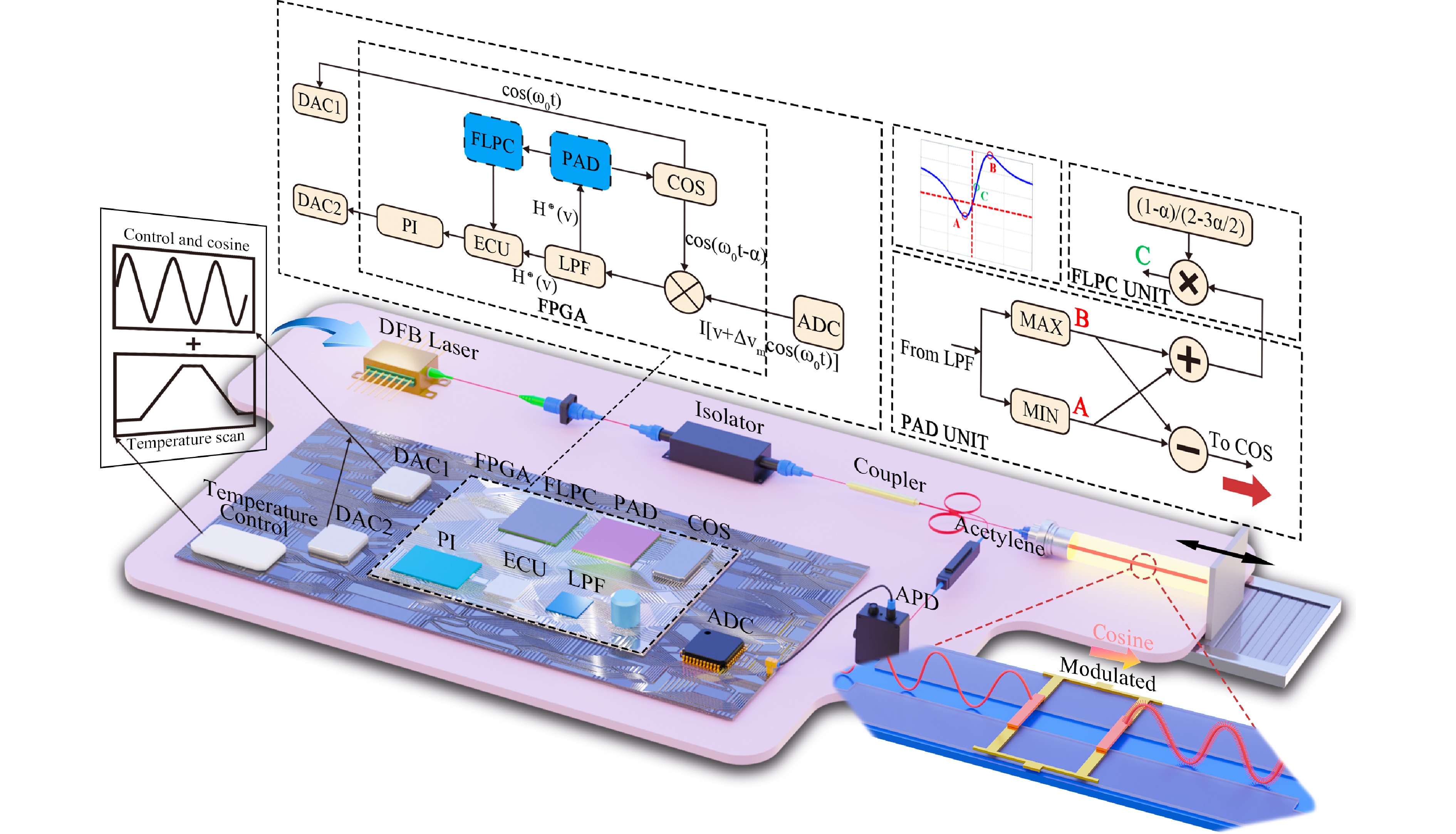
Fig. 5 Schematic of large-amplitude and high-bandwidth frequency modulation and central frequency stabilization of laser source in FMS. DFB: distributed feedback laser; Acetylene: acetylene saturation chamber; ADC: analog-to-digital converter; APD: avalanche photodetector; COS: cosine signal generating unit; PAD: peak amplitude detection unit; FLPC: frequency lock point calculation unit; LPF: low-pass filter; ECU: error calculating unit; PI: proportional-integral controller; DAC1 and DAC2: digital-to-analog converter 1 and 2.

Fig. 9 Performance evaluation of FMS to realize sub-nanometer measurements. FC: fiber circulator; FOA: fiber optic attenuator; APD: photodetector; ADC: analog-to-digital converter; DDS: direct digital frequency synthesis; LPF: low-pass filter; FPGA: field-programmable gate array; USB: universal serial bus; DAC: digital-to-analog converter. a Periodic nonlinear error test results of FMS before system optimization. b Periodic nonlinear error test results of FMS after system optimization. c Displacement resolution test results of FMS. d Static displacement stability comparison test of FMS. Red line corresponds to unoptimized frequency stabilization system, blue line to optimized frequency stabilization system.
-
To explore the relationship between the measurement performance and laser characteristics, the demodulation errors of the FMS with different modulation amplitudes at the working distance of 4.0 cm and 2.4 cm were calculated. The phase modulation depths C corresponding to different modulation amplitudes when WD = 2.4 cm were calculated according to Eq. 2. The Lissajous figures generated by the two orthogonal signals are shown in the top row of Fig. 6. The five graphs at the bottom of Fig. 6 respectively test the four modulation amplitudes of 0.50 GHz, 0.80 GHz, 1.00 GHz and 1.57 GHz for WD = 4 cm (red dashed lines), and the five modulation amplitudes of 0.50 GHz, 0.80 GHz, 1.00 GHz, 1.57 GHz and 2.62 GHz for WD = 2.4 cm (solid blue lines). The five Lissajous figures correspond to the ideal case (circle, pink line) and the actual case (ellipse, blue line), respectively.

Fig. 6 Influence of laser modulation amplitude on measurement accuracy.
By analyzing the top and bottom plots of Fig. 6, we can draw the following conclusions:
(1) As can be seen in the bottom figures, when $ \mathrm{\Delta }{\nu }_{m} $ is too small, the C value cannot be 2.63. At this time, the demodulation system will produce periodic nonlinear errors and the corresponding Lissajous figure will be an ellipse.
(2) However, when $ \mathrm{\Delta }{\nu }_{m} $ = 1.57 GHz at WD = 4 cm, and $ \mathrm{\Delta }{\nu }_{m} $ = 2.62 GHz at WD = 2.4 cm, the C value is 2.63. At this time, as demonstrated by the red dashed line in the fourth picture and the blue solid line in the fifth picture, the nonlinear error of the system is almost 0. In addition, the actual case ellipse in the fifth Lissajous curve essentially coincides with the ideal circle. This also confirms the PGC demodulation principle, i.e., when the value of C makes J1(C) and J2(C) equal, the two orthogonal signals are of equal amplitudes and the demodulation error can be minimized.
(3) Comparing the blue solid lines and the red dashed lines in the bottom figures, it is found that under the same $ \text{Δ}{\text{ν}}_{\text{m}} $, the reduction of WD will lead to a larger nonlinear error. In addition, compared to the red dashed line in the fourth figure and the blue solid line in the fifth figure, it can be seen that to reduce the nonlinear error, the smaller WD, the larger the $ \text{Δ}{\text{ν}}_{\text{m}} $ value is required. This can be explained by referring to Eq. (2) and the Bessel functions, where it can be seen that the value of C increases with the increase in WD, while the difference between J1(C) and J2(C) decreases with the increase in C until C takes the value of 2.63. Therefore, for a narrower measurement space, a larger modulation amplitude can effectively reduce the demodulation error.
(4) As can be seen in the top Lissajous figures, with the increase in C, the ellipses gradually approach the perfect circles. This also shows that the system must be under large-amplitude modulation, the two orthogonal signals will have the equal amplitudes and the measurement accuracy will be higher.
To sum up, in order to achieve a high measurement accuracy, a large-amplitude modulation must be applied. To further verify this conclusion, we compared the nonlinear error and measurement speed of several systems with different modulation amplitudes and modulation bandwidths. The comparison results are listed in Table 1, where it can be seen that the proposed method has a higher modulation bandwidth by a factor of more than 3 and a larger modulation amplitude by a factor of 4 compared to the rest. Therefore, the measurement speed be improved by more than 3 times and the nonlinear error can be reduced to the sub-nanometer level.
Method f0 $ \Delta {\nu _m} $ FMS measurement speed FMS nonlinear error (WD = 4 cm) [21] Low (< 116 kHz) Small (< 0.4 GHz) < 58 kHz > 10 nm [22] Low >(300 kHz) Small (25 MHz) 150 kHz > 10 nm Proposed High (1 MHz) Large (1.57 GHz) 500 kHz < 1 nm Table 1. Performance comparison of systems with different modulation amplitudes and bandwidths
-
To verify the theoretical derivations and model presented in Section 2, the laser wavelength was set to scan the neighborhood of the absorption peak to be locked, the frequency discrimination signal calculated in FPGA was collected, and the frequency discrimination curve was plotted in Fig. 7a using the dark blue line for $ \alpha $ = 0°. To prevent the effects of laser light intensity during scanning, temperature scanning was used for laser wavelength scanning in this experiment. The selected scanning voltage range is from −1.5 V to 1.5 V and its scanning temperature range is from 24 ℃ to 26 ℃. The range of frequency scan output voltage that produced complete frequency discrimination curves was intercepted and plotted in Fig. 7, where it can be observed that all curves were asymmetric, which was consistent with the results discussed in Section 2. These experiments demonstrated the effectiveness of the proposed model.
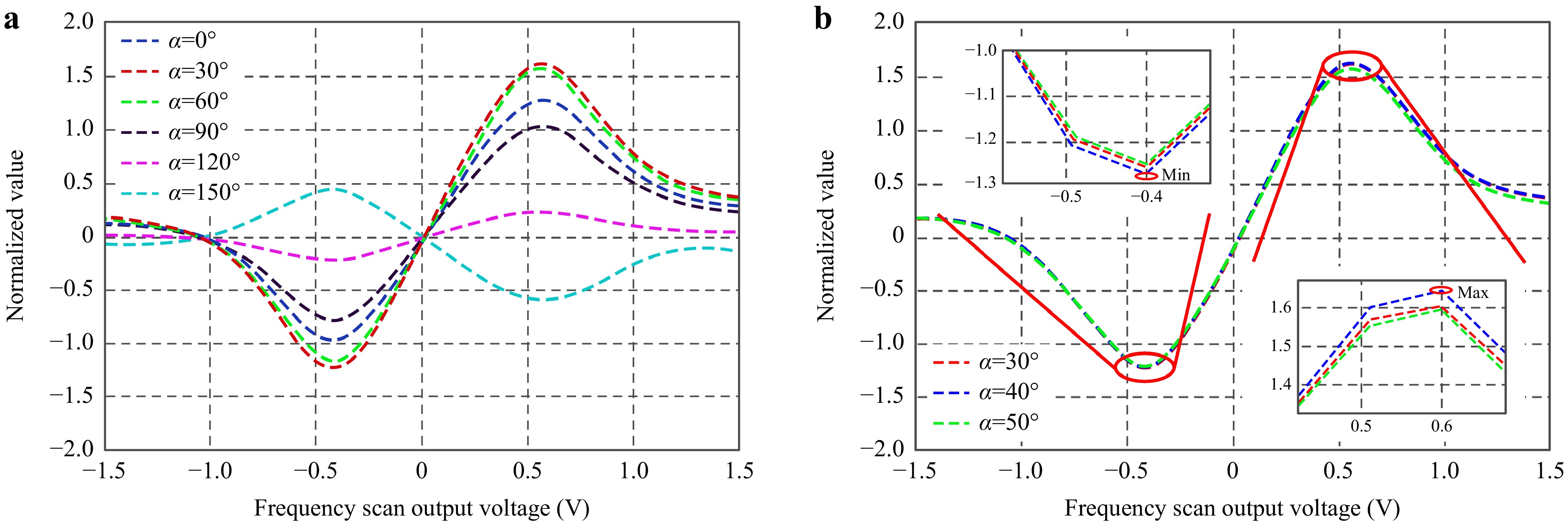
Fig. 7 Frequency discrimination curves of large-scale adjustable frequency FMS light source. a Frequency discrimination curves under stride phase adjustment and b Frequency discrimination curves under fine phase adjustment.
Fig. 7a, b correspond to the CPD compensation steps of 30° and 10°, respectively, and verify the validity of the optimization methods for eliminating the effects of CPD and AOIM on frequency discrimination curve in laser frequency stabilization systems. First, the phase of the carrier signal inside the FPGA was changed in 30°-steps from 0° to 180°. At the same time, the light source wavelength was scanned and the obtained frequency discrimination signals were drawn in Fig. 7a. The maximum and minimum values in the curve were extracted. By calculating the difference between the maximum and the minimum value, two groups of corresponding carrier signal phases with larger difference were selected, and the carrier signal phase was subdivided into 10° intervals between the extracted two phases. The above operations were repeated and the frequency discrimination signals were drawn in Fig. 7b. The CPD compensation phase with the largest difference was selected to compensate the final system. The new locking point was calculated using Eq. 21 to realize the operation of the laser frequency stabilization system.
-
Fig. 8 shows the experimental results for the laser modulation amplitude of 2.61 GHz and the laser modulation bandwidth of 1 MHz. The purpose of this part was to test the central frequency stability of the laser source optimization system for the FMS using a well-established method17.
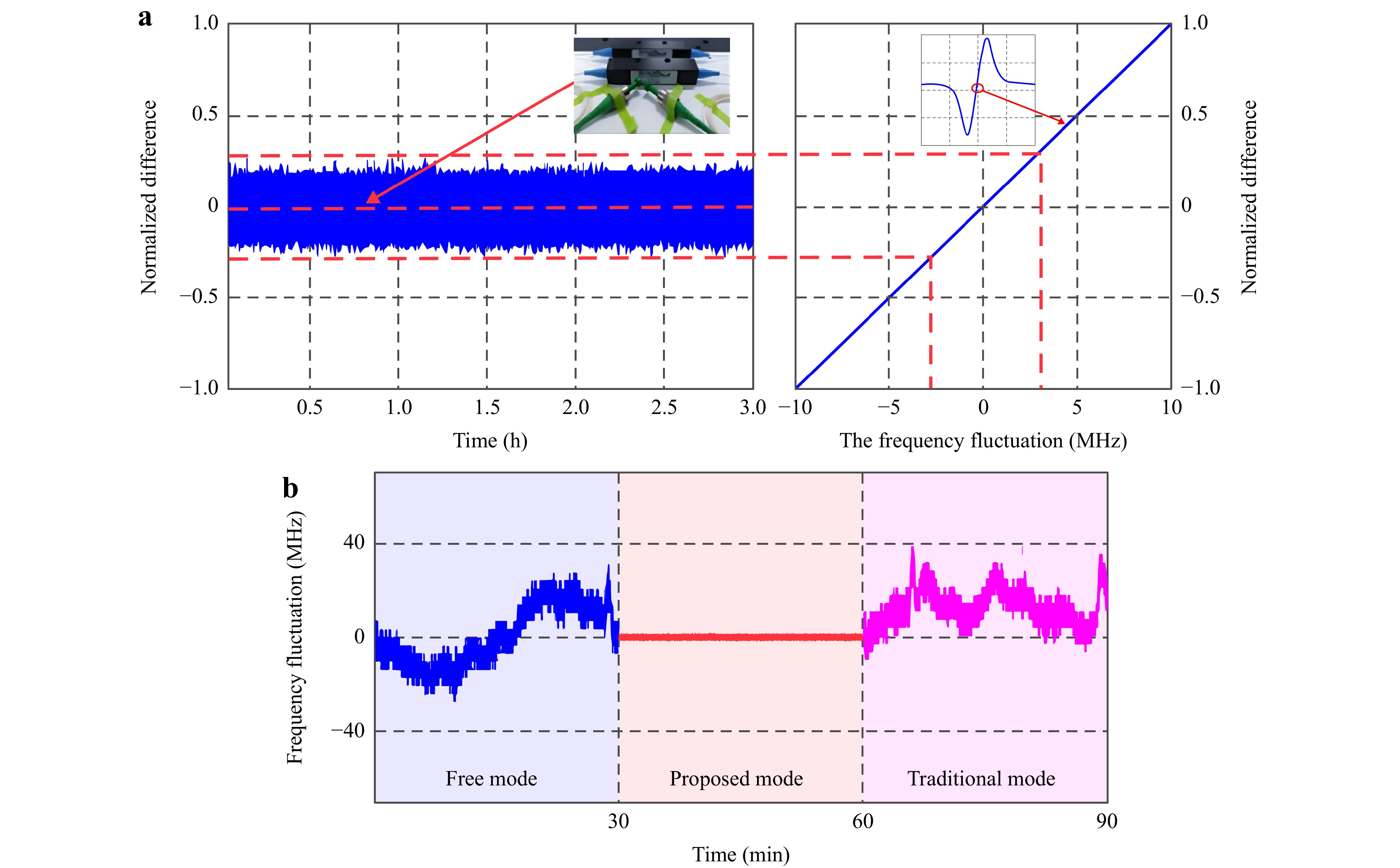
Fig. 8 Experimental results of central frequency stabilization for FMS. a Frequency locking effect and frequency fluctuations in optimized frequency stabilization system observed within 3 hours. b The frequency fluctuation results were observed continuously for 30 min in each of the three cases: blue plot corresponds to free mode, red plot to using proposed frequency stabilization method (proposed mode), and pink plot to traditional frequency stabilization method (traditional mode).
During the measurement, the system after frequency stabilization was placed in a quiet testing space and the identification frequency signals from a phase-locked amplification unit were collected for 3 h. Next, the identification frequency curve obtained by scanning the laser frequency was calculated and converted, and the linear region of the identification frequency curve was fitted with a straight line, as shown in Fig. 8a. The obtained curves were normalized and the fluctuation range of laser frequency was obtained. In Fig. 8b, the observed frequency fluctuations within 30 min in three cases of free operation, optimized frequency stabilization method and traditional frequency stabilization method are shown. The relative stability of the laser wavelength corresponding to the fluctuation peak can be obtained by converting the obtained frequency fluctuation range Δf as follows:
$$ \frac{{\Delta f}}{f} = \frac{{\Delta \lambda }}{\lambda } = \frac{{\Delta f \cdot \lambda }}{{\text{c}}} $$ (22) As can be seen from the results of Fig. 8a, the relative expanded uncertainty of the optimized laser wavelength was demonstrated to be superior to 5 × 10⁻⁸ (k = 2) within 3 hr, while the pink curve in Fig. 8b shows that when the traditional method was adopted, the system had a trouble in frequency locking at the frequency stabilization point, and the stability of the laser center frequency was 5 × 10⁻⁷. In other words, the stability of the optimized system was one order of magnitude higher than that of the traditional method, which demonstrates the effectiveness of the optimized system proposed in this paper. In addition, Fig. 8b further proves that the optimized method proposed in this paper ensures that the stable locking frequency point can be found every time to achieve high-precision laser frequency stability.
Five frequency stability calculations were carried out using the Allan variance at sampling times of 0.1 s, 1 s, 10 s, 100 s and 1,000 s respectively, and the results are listed in Table 2. The experimental results show that the achieved laser wavelength stability of the optimized system was better than 2.9 × 10⁻¹⁰ (at a sampling time τ = 1 s).
Sampling time τ (s) 0.1 1 10 100 1,000 Frequency stability according to allan variance 2.8 × 10⁻¹⁰ 2.9 × 10⁻¹⁰ 1.1 × 10⁻¹⁰ 4.1 × 10⁻¹¹ 2.5 × 10⁻¹¹ Table 2. Experimental measurements of laser wavelength stability
-
To further evaluate the performance of model and method proposed in this paper, an FMS system was built, as shown in Fig. 9. The performance evaluation experiment included a nonlinear error test, an FMS resolution test and a measurement stability test. The experimental results are plotted in Fig. 9.
First, following the nonlinear error test method proposed by the researchers15, a periodic nonlinear error test experiment was carried out on an object driven to move at a constant speed. The displacement residual was analyzed by FFT and the amplitude of the integer multiple of the corresponding motion frequency was taken as the periodic nonlinear error. As can be seen from the results in Fig. 9a, when the unoptimized system was used for the measurement, a nonlinear error of tens of nm occurred at the first and third harmonics. For comparison, the measurement results using the proposed model were plotted in Fig. 9b. There are no obvious peaks at the integer multiples of the object motion frequency and the maximum error is less than 0.8 nm, which demonstrates the potential of FMS to achieve sub-nanometer measurement accuracy.
Further, the round-trip step resolution test of the FMS was carried out, with the results shown in Fig. 9c. The step magnitude of the platform was set to 0.4 nm and 1 nm, and the step time to 0.5 s. The black line represents the displacement of the FMS and the red line the result after filtering. The FMS using the optimized frequency stabilization system can clearly identify the step round trip displacement of 1 nm, while the step round trip step of 0.4 nm can also be distinguished. Since the calibration limit resolution of the nano-displacement table used was 0.4 nm, the displacement noise level will be superimposed in the interference signal when adopted, hence, using a more precise micro-displacement table can improve the measurements. Thus, using the optimized frequency stabilization system in FMS proposed in this paper can provide a resolution exceeding 0.4 nm.
Finally, static displacement stability comparison tests of FMS were also conducted. It can be seen from the Fig. 9d that after the laser frequency stabilization optimization, the peak-to-peak value of displacement measurement of the FMS was 0.4 nm and the corresponding time was 1 min. In comparison, before the laser frequency stabilization optimization, the peak-to-peak value of displacement measurement of laser interferometer was 4 nm and the corresponding time was also 1 min. The relationship between the two results was consistent with the laser wavelength stability experimental results, which further confirmed the reliability of the test results of laser wavelength stability.
-
FMSs are considered as the next generation of embedded high-precision sensing equipment. Compared to the traditional interferometers, they are smaller, exhibit higher integration and have better anti-interference ability. In this paper, an ultra-precision and fast FMS based on PGC demodulation was designed to realize sub-nanometer measurements. The complete model and relationship between the measurement accuracy and laser characteristics was established to fill in the theoretical gaps. To improve the measurement speed and accuracy, the system adopted the high-bandwidth and large-amplitude laser frequency modulation. Concurrently, periodic nonlinear errors of tens of nm were also eliminated at the source. Further, as the measuring scale of FMS, the laser central wavelength required stabilization to achieve high measurement stability. However, the existing frequency stabilization methods and models are only applicable to the low-bandwidth and small-amplitude frequency modulation. It is well known that there is a fundamental conflict between laser modulation and stability. To solve the problem, the mechanism of the conflict was fully analyzed and explained. As a result, a modified laser central frequency stabilization model and method based on the frequency discrimination curve reconstruction under high-bandwidth and large-amplitude modulation were proposed to achieve robust central wavelength stability. The effectiveness of the proposed stabilization method was verified experimentally. The performance of the FMS with different laser modulation bandwidths and modulation amplitudes was compared. The laser central frequency stabilization results of the traditional and the proposed method were also compared, and the performance of FMS was thoroughly tested. The results show that when the modulation bandwidth was 1 MHz and the maximum modulation amplitude was 2.61 GHz, the central relative expanded uncertainty of DFB laser wavelength was demonstrated to be superior to 5 × 10⁻⁸ (k = 2) within 3 hr, with the stability according to Allan variance is 2.9 × 10⁻¹⁰. The stability of the interferometer was better than 0.4 nm/min, the resolution of FMS better than 0.4 nm, and the nonlinear error was reduced to 0.8 nm. Thus, the sub-nanoscale displacement measurements were realized. In future, we will further improve the performance of the modified frequency stabilization system and FMS to realize embedded measurements in different practical settings.
-
This research was supported by the National Key Research and Development Projects of China (No. 2022YFF0705802), National Natural Science Foundation of China (62305090), China Postdoctoral Science Foundation (2023M730883) and Fellowship of China National Postdoctoral Program for Innovative Talents (BX20230478).
Focus on sub-nanometer measurement accuracy: distortion and reconstruction of dynamic displacement in a fiber-optic microprobe sensor
- Light: Advanced Manufacturing , Article number: (2024)
- Received: 30 December 2023
- Revised: 28 August 2024
- Accepted: 29 August 2024 Published online: 18 October 2024
doi: https://doi.org/10.37188/lam.2024.051
Abstract: We established a complete model and relationship between laser source characteristics and measurement accuracy of high precision fiber microprobe sensor (FMS) based on phase generated carrier demodulation. The laser carried out high-bandwidth frequency modulation to improve the measurement speed. Meanwhile, the laser also carried out large-amplitude frequency modulation to eliminate tens of nanometers of nonlinear error, thus improving the measurement accuracy. Further, the laser center wavelength is required to be stabilized under the above modulation to achieve a high measurement stability. The conflict between laser frequency modulation and central stability is revealed and analyzed alongside the distortion of measurement accuracy. A modified frequency stabilization method for laser source under high-bandwidth and large-amplitude modulation is proposed for improving measurement accuracy to realize sub-nanometer precision. The experimental results showed that when the modulation bandwidth was 1 MHz and maximum modulation amplitude was 2.61 GHz, the distributed feedback laser central wavelength stability was 2.9 × 10⁻¹⁰ (τ = 1s) according to Allan variance. Additionally, the relative expanded uncertainty of the laser wavelength was demonstrated to be superior to 5 × 10⁻⁸ (k = 2) within 3 hr, which was at least one order of magnitude higher than that of the traditional method. The resolution and stability of FMS is better than 0.4 nm, and the nonlinear error is reduced from tens of nm to 0.8 nm, which meets the requirements of sub-nanometer measurements.
Rights and permissions
Open Access This article is licensed under a Creative Commons Attribution 4.0 International License, which permits use, sharing, adaptation, distribution and reproduction in any medium or format, as long as you give appropriate credit to the original author(s) and the source, provide a link to the Creative Commons license, and indicate if changes were made. The images or other third party material in this article are included in the article′s Creative Commons license, unless indicated otherwise in a credit line to the material. If material is not included in the article′s Creative Commons license and your intended use is not permitted by statutory regulation or exceeds the permitted use, you will need to obtain permission directly from the copyright holder. To view a copy of this license, visit http://creativecommons.org/licenses/by/4.0/.

 DownLoad: