Generation of polarization-multiplexed terahertz orbital angular momentum combs via all-silicon metasurfaces

Orbital angular momentum (OAM), as an inherent feature of electromagnetic waves (EM waves) with additional degrees of freedom¹, has attracted plenty of interest during the past several decades. The beams carrying OAM, also known as vortex beams or OAM beams, possess vortex wavefront which is defined by topological charge¹. Different OAM modes have different topological charges. Mathematically, OAM beams with different OAM modes remain orthogonality. So, multi-mode OAM beams can increase channel capacity because of the mode orthogonality². Due to this unique advantage, various applications have emerged, such as super-resolution imaging³, optical trapping⁴, quantum information processing⁵, multi-channel communications^6,7, and holography⁸. Currently, enormous methods have been reported to generate OAM beams, including diffractive optical elements⁹, antenna arrays¹⁰, liquid crystals¹¹, and nanosieves¹². However, most reported schemes can only generate single or several simple OAM modes, preventing from flexibly manipulating a series of equally spaced OAM channels with the same intensities, i.e., OAM comb¹³.

On the other hand, metasurfaces, composed of subwavelength planar microstructures (namely meta-atoms), are extremely fascinating for their features of compact footprints and strong capabilities to manipulate EM waves¹⁴. By tuning the spacial size of every meta-atom, the phase delay of transmitted (or reflected) EM waves can be flexibly controlled. At the same time, because of the strong anisotropy of meta-atoms, the phase delay usually differs in different incident polarizations¹⁵. In this way, many schemes have been put forward to control surface waves^16–19, generate holograms^20–23, generate OAM beams^24–26, manipulate polarization states^27–30, and produce upconversion photoluminescence³¹. Therefore, metasurfaces are promising candidates for generating polarization-multiplexed wavefront that suits pre-designed functions, including OAM combs. Utilizing metasurfaces, arbitrary polarization-multiplexed OAM combs can be flexibly designed. The OAM combs that contain many orthogonal different OAM modes may be transmitted as a carrier wave in a communication link, such as a wireless THz communication link, providing a promising scheme for an arbitrary multi-mode communication system^32,33.

In this paper, we propose, fabricate, and characterize two categories of metasurfaces that can realize the generation of polarization-multiplexed OAM combs working in the terahertz (THz) range. As shown in Fig. 1, the metasurfaces consist of an array of silicon pillars, the sizes of which along the x-direction and y-direction can be independently tuned to produce different propagation phases, thus creating a carefully designed wavefront for both x-polarized and y-polarized (x-pol and y-pol) incident waves simultaneously. In this way, the modulated wavefront can ultimately form an OAM comb on the focal plane. As a proof of concept, we first design a metasurface to generate a pair of polarization-multiplexed OAM combs with arbitrary lengths, which means that OAM mode numbers within the OAM combs can be arbitrarily controlled. Furthermore, another metasurface is proposed to realize a pair of polarization-multiplexed OAM combs with arbitrarily controlled locations and intervals in the OAM spectrum. Experimental results agree well with full-wave simulations, validating a good performance of OAM combs generation. Our scheme may open a new door to designing high-capacity THz communication devices.

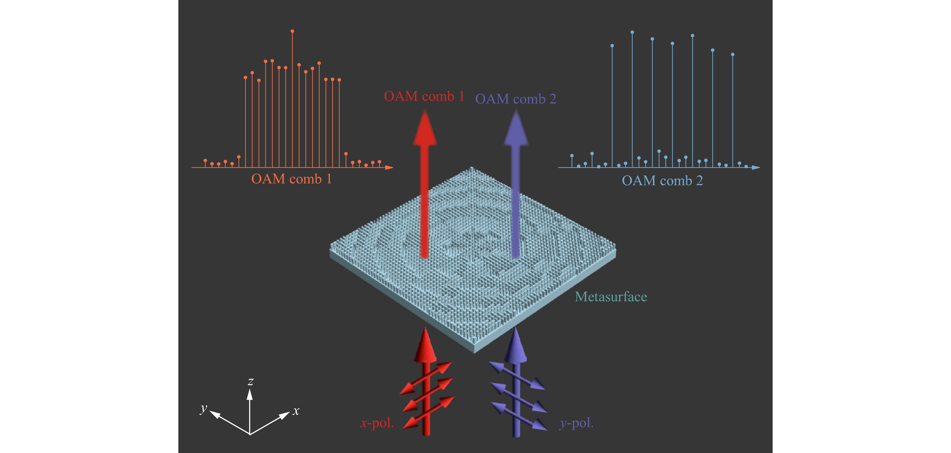
Fig. 1  Schematic of the proposed metasurface for the generation of polarization-multiplexed OAM combs, constructed by silicon pillars as meta-atoms above the silicon substrate. The x-pol and y-pol incident waves normally shine the metasurface and are then converted to OAM comb 1 and 2 on the focal plane, respectively.

Here, we adopt rectangular silicon pillars and a silicon substrate to construct a transmission-type metasurface, as shown in Fig. 1 and 2a. Each silicon pillar can be regarded as a birefringent scatterer which modulates the complex amplitude of the transmitted EM waves along its long and short axes differently. When the long/short axis is along the x-/y-direction, its transmissive feature can be described as:

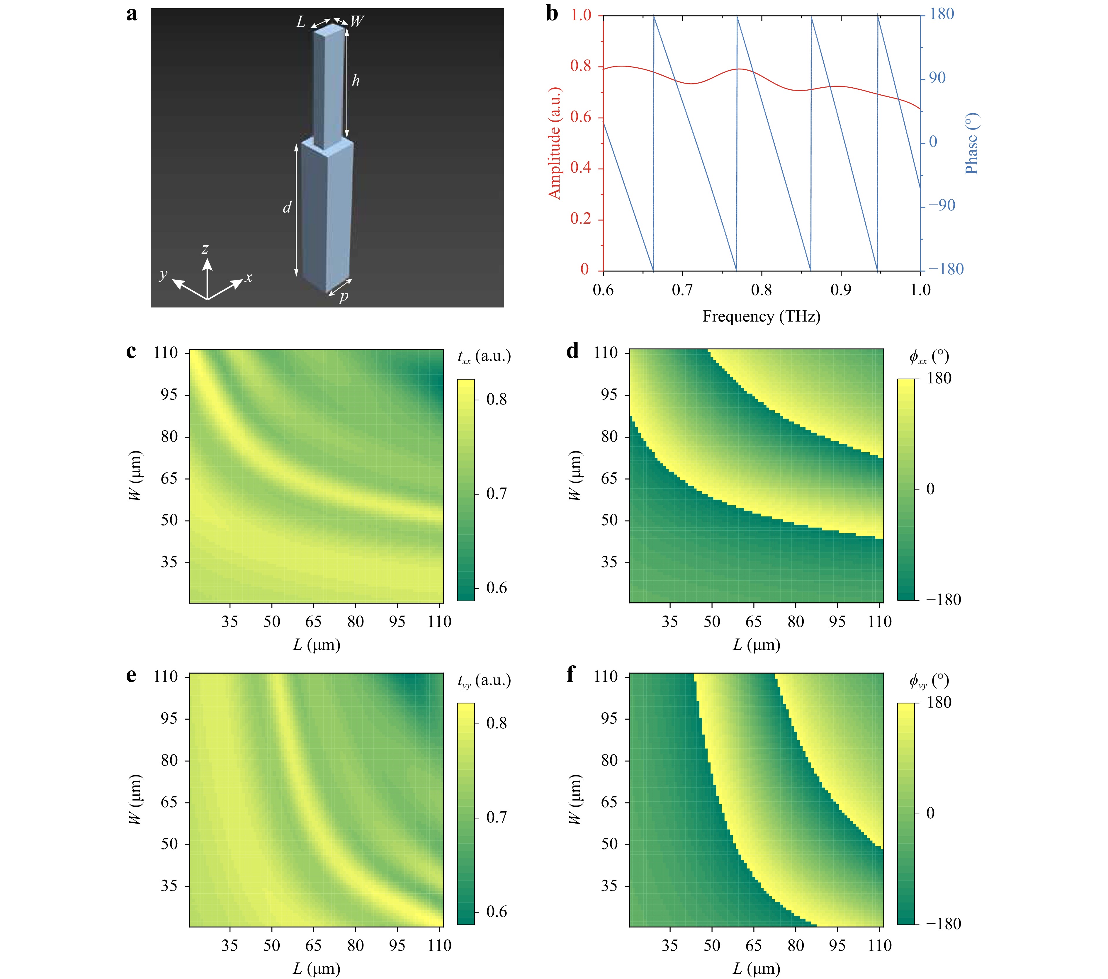
Fig. 2  a Schematic of a designed meta-atom. b Simulated transmission amplitude and phase spectrum of a meta-atom with L = 60 μm and W = 80 μm, under x-pol incidence. c−f Simulated transmission c, e amplitudes and d, f phases under c, d x-pol and e, f y-pol incidences with different L and W at 0.8 THz.

where ${T_{xx}} = {t_{xx}}{e^{i{\phi _{xx}}}}$ and ${T_{yy}} = {t_{yy}}{e^{i{\phi _{yy}}}}$ are transmission coefficients under x- and y-polarized incidence. Then the transmitted field can be given as:

where there is no polarization transformation. In this way, the transmitted x- and y-pol fields can be simultaneously modulated by changing the transmissive feature of every meta-atom.

To properly suit the working frequency (0.8 THz), the parameters of meta-atoms are carefully chosen, including period p = 120 μm, height h = 400 μm, substrate thickness d = 600 μm, with length L and width W varying from 20 μm to 110 μm (see Section A, Supplementary Information). Afterward, we implement full-wave simulations using the commercial software CST Microwave Studio 2021 (see more details in the Numerical Simulation Section, Methods). A meta-atom’s transmission amplitude and phase spectrum with L = 60 μm and W = 80 μm are simulated under x-pol incidence (Fig. 2b), showing a high transmission amplitude from 0.6 THz to 1.0 THz. At the working frequency of 0.8 THz, L and W are swept from 20 μm to 110 μm to calculate the corresponding transmission amplitudes and phases under x-pol and y-pol incidence, shown in Fig. 2c–f. It can be seen when L and W change, the amplitudes remain high and stable (above 0.6 and below 0.8), while phases cover the whole 360° range for each polarization. In this way, we select 144 meta-atoms with a phase gradient of 30° to cover the phase range of 0−360° for both x-pol and y-pol incident waves. It is worth noting that the phase gradient of 30° can theoretically provide higher accuracy, while simultaneously satisfying the calculation and fabrication allowance (with more details in Section A, Supplementary Information).

To realize the designed function, the meta-atoms need to exhibit the following phase distributions:

Here, (r, θ) is the in-plane position in the polar coordinate system, $\phi _D^x\left( \theta \right)$ and $\phi _D^y\left( \theta \right)$ represent the Dammann phases for x-pol and y-pol incidences, ${\phi _f}\left( r \right) = - \dfrac{{2{\text π} }}{\lambda }\left( {\sqrt {{r^2} + {f^2}} - f} \right)$ is the focusing phase to converge the transmitted waves (λ = 375 μm) into the focal plane at focus length f = 7.5 mm. Traditionally, the Dammann phase is the phase profile for Dammann gratings, a kind of binary optics element, to generate an equal-energy field distribution among all desired diffraction orders³⁴. In this work, we use the azimuthal Dammann phases to generate OAM combs, while their binary phase values (0 or π) are decided using azimuthal transition points, which can be derived from a numerical optimization method³⁵. These transition points are crucial to generate OAM combs. Then, the transmission coefficient of the first designed azimuthal Dammann phase mask can be described as:

where Λ is the azimuthal period, and C_n is the coefficient of the nth OAM mode, the value of which can be determined by azimuthal transition points. Thus, modulated by the azimuthal Dammann phase in the θ-space (Fig. 3), OAM combs that contain several OAM series with different topological charges l, are formed after EM waves pass through the metasurfaces. The focusing phase is also added to observe OAM combs on the focal plane. Theoretically, the process of OAM mode analysis can be described by the Fourier transform in the polar coordinate system, and then the OAM spectrum of the field on the focal plane can be written as:

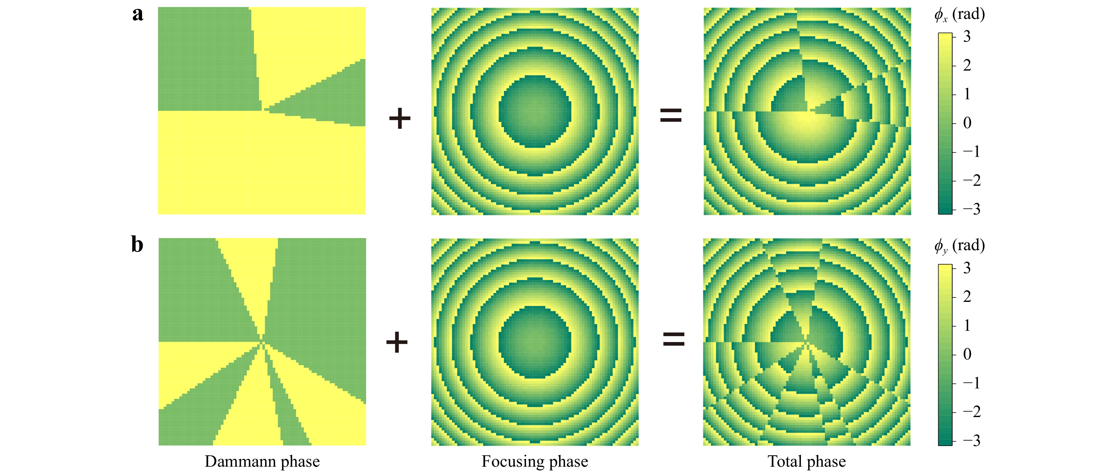
Fig. 3  a, b Schematic illustration of the process for creating phase profiles of sample 1 under a x-pol and b y-pol incidence.

where l is the topological charge of an OAM mode, $\mathcal{F}\left\{ \cdot \right\}$ denotes the Fourier transform, and $\delta \left( \cdot \right)$ represents the unit-impulse function. It is worth noting that l and θ are a pair of Fourier transform bases. In this way, the OAM comb can be realized on the focal plane by selecting a series of transition points, which determine the values of different C_n. To be specific, in Fig. 3a, the transition points are θ_n = {0, 0.23191, 0.42520, 0.52571, 1} × 2π to generate an OAM comb with l = {–3, –2, …, +3}. By contrast, in Fig. 3b, the transition points are θ_n = {0, 0.18240, 0.27424, 0.58581, 0.67967, 0.71917, 0.82217, 0.90642, 1} × 2π to generate an OAM comb with l = {–7, –6, …, +7}. In the two cases, Λ = 2π.

Then we fabricate the first sample through the deep reactive ion etching (DRIE) process (see more details in the Sample Fabrication Section, Methods), the photo of which is demonstrated in Fig. 4a. Sample 1 contains 80 × 80 rectangular silicon pillars as meta-atoms with a total size of 9.6 mm × 9.6 mm (with more details in Section B, Supplementary Information). Next, a THz near-field scanning system is adopted to characterize the function of sample 1, as schematically shown in Fig. 4b. The x-pol (or y-pol) incident waves normally shine sample 1, and then the field distributions of the corresponding polarization are detected by a probe on the focal plane with z = 7.5 mm (see more details in the Experimental Setup Section, Methods). Fig. 4c and d show the simulated (in the 1st row) and the measured (in the 2nd row) x-pol (or y-pol) electric field distribution of intensity (|E_x|² or |E_y|²) and phase (ϕ_x or ϕ_y) under x-pol (or y-pol) incidence on the focal plane, suggesting that the simulated results agree with experimentally measured ones. The beams are focused on the central area, where some dark lines suggest an abrupt phase change of π. The field patterns are complicated, indicating there are multi-mode OAM waves (i.e., OAM combs). Theoretically, the electric field distributions on the focal plane (in the polar coordinate system) can be denoted by the superposition of vortex harmonics $\exp \left( {il\theta } \right)$:

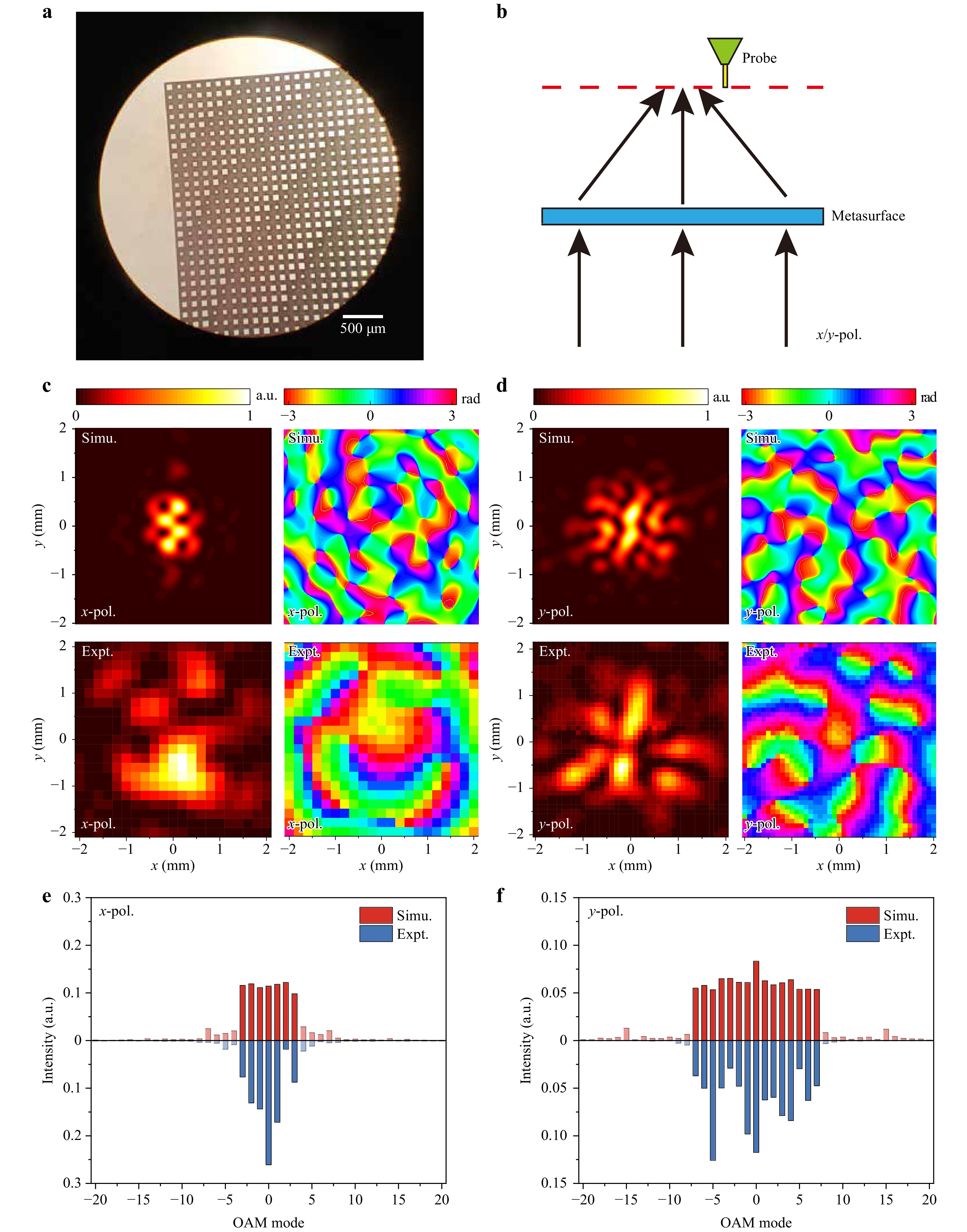
Fig. 4  a A photo of part of the fabricated sample 1. b Schematic of the THz field measurement process. c, d Simulated (in the 1st row) and measured (in the 2nd row) field distributions of intensity and phase under c x-pol and d y-pol incidence on the focal plane of sample 1. e, f Calculated OAM spectrum by analyzing simulated and measured field distributions on the focal plane of sample 1 under e x-pol and f y-pol incidence.

where the complex weights ${a_l}\left( r \right)$ can be calculated by:

Then the intensity of OAM modes l can be described as:

Using Eq. 7 and 8, We can analyze the simulated and measured field distributions $E\left( {r,\theta } \right)$ at each location $\left( {r,\theta } \right)$ in the polar coordinate system. Then the normalized calculated mode intensities ${P_l} = {{{A_l}} \mathord{\left/ {\vphantom {{{A_l}} {\displaystyle\sum\limits_{l = - \infty }^{ + \infty } {{A_l}} }}} \right. } {\displaystyle\sum\limits_{l = - \infty }^{ + \infty } {{A_l}} }}$ under x-pol (or y-pol) incidence are depicted in Fig. 4e and f. As theoretically predicted, these fields are the superposition of a series of OAM modes with equal intensities (i.e., OAM combs). The x-pol (or y-pol) incident waves passing through sample 1 can be converted to an OAM comb with l from –3 to +3 (or from –7 to +7), whose length is 7 (or 15). As a result, a pair of polarization-multiplexed OAM combs with different lengths are achieved. The experimental results agree with the simulation. However, there is still some deviation between them. We attribute the causes to the limit of the fabrication and measurement processes, with more details in Section C, Supplementary Information.

Similarly, the meta-atoms for the second function need to possess the following phase distributions:

where $\phi _v^{x,y}\left( \theta \right) = l_0^{x,y}\theta $ denotes the vortex phase with a topological charge l₀ for x-pol or y-pol incidence. Specifically, $l_0^x = + 3$ and $l_0^y = + 2$. Compared with the last section, the vortex phase is added to the total phase distribution. Then the transmission coefficient of the second designed azimuthal phase mask can be written as:

After incorporating the focusing phase, on the focal plane, the OAM spectrum of the field can be analyzed by:

In this way, the OAM comb can be formed on the focal plane by selecting l₀, Λ, and a series of transition points. To be specific, in Fig. 5a, l₀ = +3, Λ = π, and the transition points are θ_n = {0, 0.11596, 0.21260, 0.26286, 0.50000, 0.61596, 0.71260, 0.76286, 1} × 2π to generate an OAM comb with l = {–3, –1, +1, +3, +5, +7, +9}. By contrast, in Fig. 5b, l₀ = +2, Λ = 2π/3, and the transition points are θ_n = {0, 0.07730, 0.14173, 0.17524, 0.33333, 0.41064, 0.47507, 0.50857, 0.66667, 0.74397, 0.80840, 0.84190, 1} × 2π to generate an OAM comb with l = {–7, –4, –1, +2, +5, +8, +11}. It can be easily seen that in the OAM spectrum, the location is l₀, while the interval is 2π/Λ.

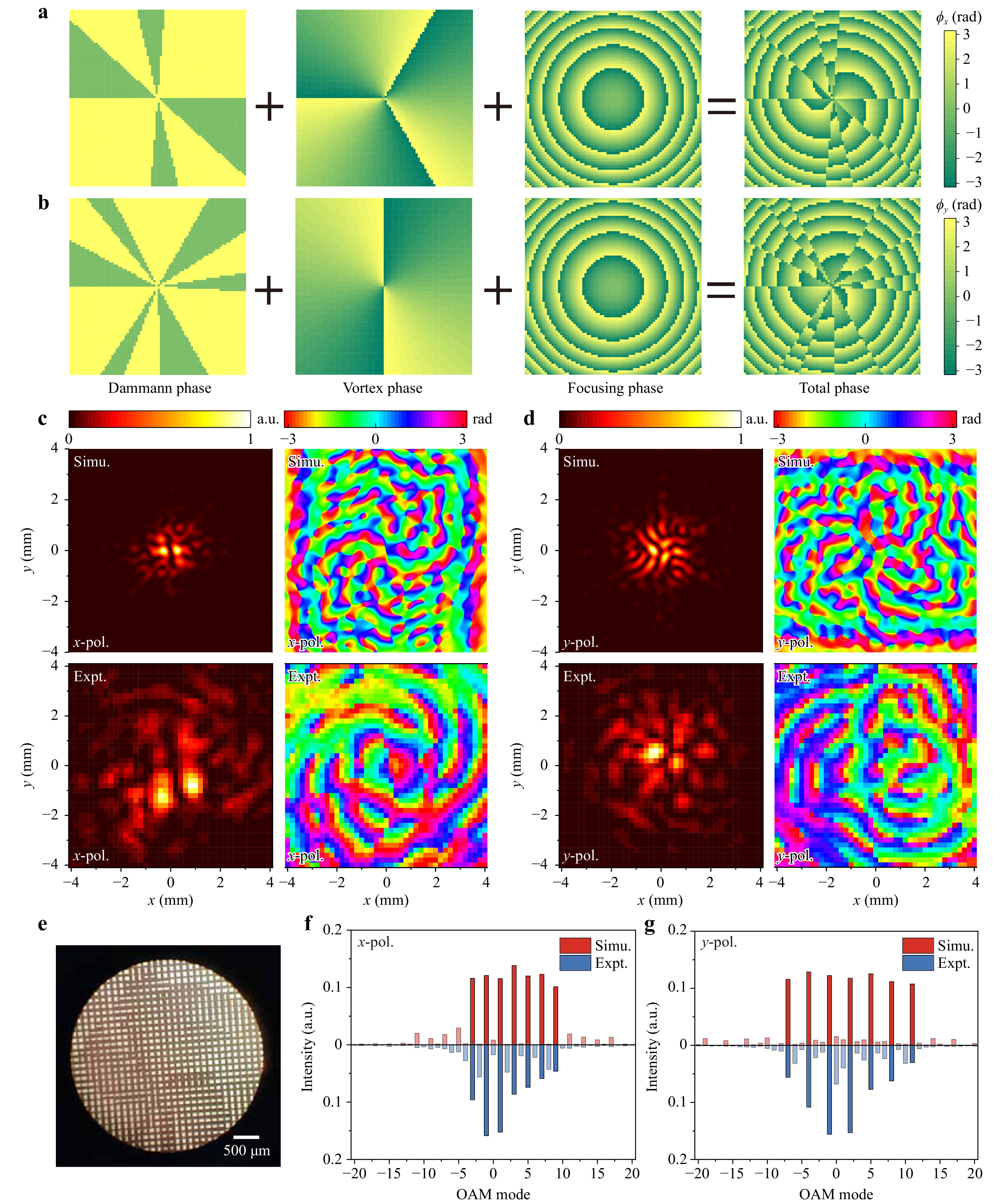
Fig. 5  a, b Schematic illustration of the process for creating phase profiles of sample 2 under a x-pol and b y-pol incidence. c, d Simulated (in the 1st row) and measured (in the 2nd row) field distributions of intensity and phase under c x-pol and d y-pol incidence on the focal plane of sample 2. e A photo of part of the fabricated sample 2. f, g Calculated OAM spectrum by analyzing simulated and measured field distributions on the focal plane of sample 2 under f x-pol and g y-pol incidence.

We then fabricate the second sample using the DRIE process, the photo of which is shown in Fig. 5e, with the same size as sample 1 (see more details in Section B, Supplementary Information). Next, the function of sample 2 is experimentally measured using the same measurement process shown in the last section. Fig. 5c and d demonstrate the simulated (in the 1st row) and the measured (in the 2nd row) x-pol (or y-pol) electric field distribution of intensity (|E_x|² or |E_y|²) and phase (ϕ_x or ϕ_y) under x-pol (or y-pol) incidence on the focal plane, suggesting a good agreement between simulated results and experimentally measured ones. After analyzing the field distributions, the normalized calculated mode intensities under x-pol and y-pol incidence are shown in Fig. 5f and g. As theoretically predicted, these fields are OAM combs. The x-pol (or y-pol) incident waves passing through sample 2 can be converted to an OAM comb with l = {–3, –1, +1, +3, +5, +7, +9} (or l = {–7, –4, –1, +2, +5, +8, +11}). Obviously, in the OAM spectrum, the location of the x-pol (or y-pol) OAM comb is +3 (or +2), while the interval is 2 (or 3). As a result, a pair of polarization-multiplexed OAM combs with different locations and intervals are achieved. The reasons for the deviation between measured and simulated results can be found in Section C, Supplementary Information.

Some schemes have been reported to realize the generation of OAM combs, but our method has its unique advantage. Compared with the work achieved by shape-tailored metasurfaces²⁴, our scheme based on the azimuthal Dammann phase can improve the capacity of OAM modes. In addition, compared with the method realized by bulky spatial light modulators (SLMs)³⁶, our metasurfaces-based scheme can make the devices more compact, and at least double the theoretical capacity of OAM channels through polarization-multiplexing. Besides, the all-silicon configuration makes the devices easy to fabricate, thus saving the manufacturing cost.

To conclude, we propose a scheme to design metasurfaces that can realize the generation of polarization-multiplexed OAM combs working in the THz range. Utilizing the principle of propagation phases, the wavefront for both x-pol and y-pol incident waves can be manipulated simultaneously, which can ultimately form an OAM comb on the focal plane. As a proof of concept, we first design a metasurface to generate a pair of polarization-multiplexed OAM combs with arbitrary mode numbers. Furthermore, another metasurface is proposed to realize a pair of polarization-multiplexed OAM combs with arbitrary locations and intervals in the OAM spectrum. Experimental results and full-wave simulations are in good agreement, suggesting a great performance of OAM combs generation. Our strategy may provide a new solution to designing high-capacity THz communication devices by introducing multi-mode and dual-polarization configurations.

All simulations are implemented using the commercial software CST Microwave Studio (version 2021.1). The dielectric constant of silicon is ε_r = 11.9. A plane wave (x-pol or y-pol) is defined as the source. The transmission amplitudes and phases of meta-atoms are simulated by the Time Domain Solver. The periodic boundary condition is applied in both the x- and y-directions, while the open boundary condition is utilized in the z-direction. A probe is set 400 μm above the metasurface to detect the transmission coefficient. The sizes of a meta-atom are swept to establish a database of the transmission coefficient, where we select 144 meta-atoms to match the phase gradient of 30° (with more details in Section A, Supplementary Information). Then these meta-atoms are applied to construct our metasurfaces according to the pre-designed phase profiles. As for the entire metasurfaces, open boundary conditions are applied in the x-, y-, and z-directions. The field distributions can be obtained by setting field monitors at the working frequency.

The samples are fabricated using the deep reactive ion etching (DRIE) process (also called as Bosch process). A high-resistance silicon wafer (N-type, <100>) with a thickness of 1 mm and a diameter of 4 inches is chosen as the raw material. First, the wafer is cleaned using the ultrasonic method (with acetone and isopropyl alcohol) for 5 minutes. Next is the lithography process (the machine is SUSS-MA8). The photoresist (AZ4620, with a thickness of about 6.8 μm) is spin-coated (4000 rpm, 30 seconds) on the top of the wafer, which is then baked at 100 ℃ for about 150 seconds. Then the wafer is exposed to UV light through a pre-designed mask and then goes through the development process using TMAH developer (25% TMAH: water = 1: 8, 90~120 seconds). Next, the wafer is etched by the DRIE technique (with etching gas of SF₆ and passivation gas of C₄F₈). The etching depth is 400 μm (with an error of ±20 μm). Then, the photoresist on the wafer is removed using a wet cleaning table (hydrogen peroxide: concentrated sulfuric acid = 1:3). Finally, the wafer is cut to obtain several samples.

The measured field distributions are obtained using a THz near-field scanning system based on the terahertz time-domain spectroscopy (THz-TDS) method (shown in Fig. 6). Both the THz source (transmitter) and probe (receiver) are based on the photoconductive antenna technique. The incident femtosecond (fs) laser with a central wavelength of 780 nm is divided into two parts: one part impinges on the THz source to radiate THz waves, while the other part is coupled into a single-mode fiber and then shines the THz probe, which is fixed on a three-dimensional (3D) translation stage to scan the field distributions on the desired plane. After scanning, the field distributions at each location are detected in the time domain. Then performing the Fourier transform, the complex field distributions (including both amplitude and phase) are obtained in the frequency domain. In this way, the amplitude and phase are simultaneously detected at the working frequency (0.8 THz).

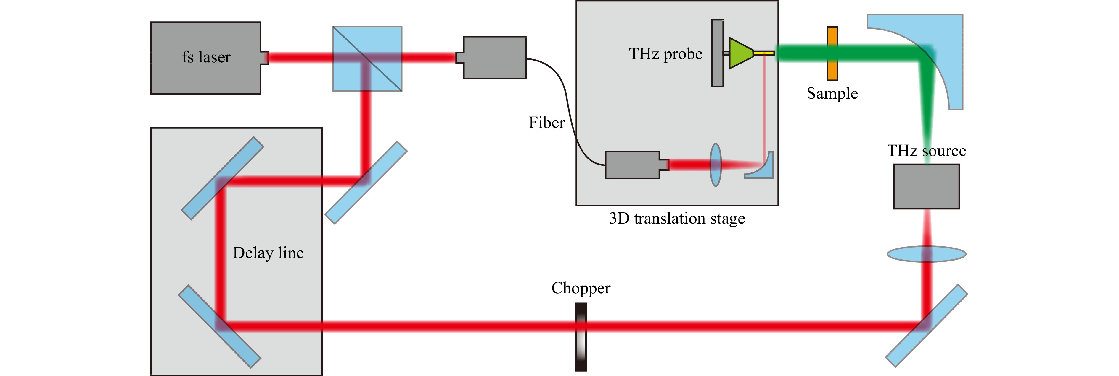
Fig. 6  Schematic of the THz near-field scanning system in our experiment.

The authors acknowledge financial support from the National Key Research and Development Program of China (No. 2019YFA0210203), and the National Natural Science Foundation of China (No. 62271011, No. 61971013).