


-
Lasers in the context of material processing are highly versatile tools that allow for the execution of a wide range of processes. Yet, determining optimal process parameters for a specific task can be exceedingly challenging due to the high-dimensional nature of the parameter space, commonly referred to as the “curse of dimensionality”1.
To address this challenge, an increasing number of machine learning algorithms are being employed2–5. One particular black box optimization method frequently applied under noisy conditions, and when the parameters to be optimized are typically fewer than 20, is Bayesian optimization (BO)6. This method has also been used in optimizing laser materials processing7–13. However, these studies often narrow their focus to specific processes.
Therefore, this paper explores the broader question of whether Bayesian optimization is applicable to real-world problems, emphasizing its generic utility for laser process developers in practical scenarios. We provide a concise introduction to Bayesian optimization, including available frameworks that simplify its use for laser process developers in practice. Furthermore, we assess its practical applicability in the contexts of laser cutting, laser polishing, and laser welding. Our research shows that sophisticated optimization frameworks, combined with modest expertise from process developers, enable the identification of adequate process parameters. This is achieved within just a few tens of experimental iterations.
Nevertheless, we recognize that in addition to modest process knowledge, a basic understanding of the underlying mathematics is crucial for achieving optimal results.
-
In order to optimize a laser process, the first step involves identifying the quality properties that need to be optimized. Subsequently, a cost function denoted as $ f_c $ is established to quantitatively relate these properties. A smaller value of $ f_c $ indicates a higher quality process. Given that the quality properties themselves are a function of the process parameters $ {\boldsymbol{x}} \in A $ originating form a parameter space $ A $, $ f_c $ is mathematically expressed as follows
$$ f_c: A \to \mathbb{R};\ \ \ {\boldsymbol{x}} \mapsto f_c \left({\boldsymbol{x}} \right) $$ (1) The goal is to find the optimal parameter $ {\boldsymbol{x}} _{\text{opt}} $, namely
$$ {\boldsymbol{x}} _{\text{opt}} : = \underset{{\boldsymbol{x}} \in A}{\arg \min}\ f_c\left({\boldsymbol{x}} \right)\ \ \ \Leftrightarrow\ \ \ {\boldsymbol{x}} _{\text{opt}} = \underset{{\boldsymbol{x}} \in A}{\arg \max} \left(- f_c\left({\boldsymbol{x}} \right) \right) $$ (2) In an experimental context, such as optimizing laser processes, the search for $ {{\boldsymbol{x}}_{\text{opt}}} $ is typically aided by conducting experiments that yield a set of data points, denoted as
$$ D_n : = \lbrace \left({\boldsymbol{x}}_1, y_1 \right),..., \left({\boldsymbol{x}}_n, y_n \right) \rbrace ; \ \ \ \ n \in \mathbb{N} $$ (3) Each data point, labeled by $ j = 1,...,n $, comprises an input parameter $ {{\boldsymbol{x}}_j} $ along with the measured $ {y_j} $ serving as an potentially noisy observation for $ {f_c\left({\boldsymbol{x}}_j\right)} $.
In the context of Bayesian optimization, the cost function $ f_c $ is approximated by a surrogate model. A commonly used surrogate model is a Gaussian process $ {f_c \sim {\cal{GP}} (m, k)} $, which also captures uncertainties in the knowledge of $ f $. The Gaussian process is defined by a mean function $ {m: A \to \mathbb{R}} $ and a covariance function or kernel $ {k: A \times A \to \mathbb{R}} $. In general, a Gaussian process is a stochastic process $ {\left \lbrace X_{{\boldsymbol{x}}} \right \rbrace_{{\boldsymbol{x}} \in I}} $ defined on an index set $ {I \subseteq A} $, which follows a multivariate normal distribution $ {{\cal{N}}({\boldsymbol{\mu}}, {\bf{\Sigma}})} $ when $ I $ is restricted to a finite subset of $ A $
$$ {\boldsymbol{X}} : = \left( X_{{\boldsymbol{x}}_1}, \ldots, X_{{\boldsymbol{x}}_n} \right)^{T} \sim {\cal{N}} \left( {\boldsymbol{\mu}}, {\bf{\Sigma}} \right);\ \ \ \ n = |I| $$ (4) Here, $ m({\boldsymbol{x}}) $ and $ k({\boldsymbol{x}}, {\boldsymbol{x}}') $ define the mean vector $ {\boldsymbol{\mu}} $ and covariance matrix $ {\bf{\Sigma}} $. When restricting $ {I = \lbrace {\boldsymbol{x}}_1,...,{\boldsymbol{x}}_n \rbrace} $ to the already experimentally evaluated input parameters described by Eq. 3, $ {\boldsymbol{\mu}} $ and $ {\bf{\Sigma}} $ are defined as follows
$$ {\boldsymbol{\mu}} : = \left( m({\boldsymbol{x}}_1),...,m({\boldsymbol{x}}_n) \right); $$ (5) $$ {\bf{\Sigma}} : = \left( {\begin{array}{*{20}{c}} { k({\boldsymbol{x}}_1, {\boldsymbol{x}}_{1}) + \epsilon^2 }&{ ... }&{ k({\boldsymbol{x}}_1, {\boldsymbol{x}}_{n})}\\ {\vdots }&{ \ddots }&{ \vdots}\\ { k({\boldsymbol{x}}_n, {\boldsymbol{x}}_{1}) }&{ ... }&{ k({\boldsymbol{x}}_n, {\boldsymbol{x}}_{n}) + \epsilon^2 } \end{array}} \right) $$ (6) Table 1 provides an overview of common kernels, with the hyperparameter $ l $ and $ \gamma $ optimized for the data at hand, which also applies to the estimated variance of the homoscedastic noise $ \epsilon^2 $.
Squared Exponential $ k({\boldsymbol{x}}, {\boldsymbol{x}}') = \exp \left( - \dfrac{1}{2 l^2} \Vert {\boldsymbol{x}} - {\boldsymbol{x}}' \Vert^2 \right) $ $\gamma$ Exponential $ k({\boldsymbol{x}}, {\boldsymbol{x}}') = \exp \left( - \left( \dfrac{\Vert {\boldsymbol{x}} - {\boldsymbol{x}}' \Vert}{l} \right)^{\gamma} \right) $ $3/2$ Matérn $ k({\boldsymbol{x}}, {\boldsymbol{x}}') = \left( 1 + \dfrac{\sqrt{3} \Vert {\boldsymbol{x}} - {\boldsymbol{x}}' \Vert}{l} \right)\exp \left( \dfrac{ - \sqrt{3} \Vert {\boldsymbol{x}} - {\boldsymbol{x}}' \Vert}{l} \right)$ $5/2$ Matérn $ k({\boldsymbol{x}}, {\boldsymbol{x}}') = \left( 1 + \dfrac{\sqrt{5} \Vert {\boldsymbol{x}} - {\boldsymbol{x}}' \Vert}{l} + \dfrac{5 \Vert {\boldsymbol{x}} - {\boldsymbol{x}}' \Vert^2}{3 l^{2}} \right)\exp \left( \dfrac{ - \sqrt{5} \Vert {\boldsymbol{x}} - {\boldsymbol{x}}' \Vert}{l} \right)$ Table 1. Common kernels $k({\boldsymbol{x}}, {\boldsymbol{x}}')$14
The advantage of approximating $ f_c $ by a probabilistic surrogate model like a Gaussian process is, that one can determine the posterior probability for $ f_c $ given the experimental data $ D_n $ by
$$ \begin{array}{l} P (f_c |D_n, {\boldsymbol{x}}) = {\cal{N}} (\mu_n ({\boldsymbol{x}}), \sigma_{n}^2 ({\boldsymbol{x}})),\ \ \ \ \text{with}\\ \ \ \ \ \ \ \mu_n ({\boldsymbol{x}}) = {\boldsymbol{k}}^T \cdot {\bf{\Sigma}}^{-1} \cdot {\boldsymbol{y}}; \\ \ \ \ \ \ \ \sigma_{n}^2 ({\boldsymbol{x}}) = k({\boldsymbol{x}}, {\boldsymbol{x}}) - {\boldsymbol{k}}^T \cdot {\bf{\Sigma}}^{-1} \cdot {\boldsymbol{k}}; \\ \ \ \ \ \ \ \ \ \ \ \ \ {\boldsymbol{k}} = \left[k({\boldsymbol{x}}, {\boldsymbol{x}}_1),..., k({\boldsymbol{x}}, {\boldsymbol{x}}_n) \right]; \\ \ \ \ \ \ \ \ \ \ \ \ \ {\boldsymbol{y}} = \left[y_1,...,y_n \right] \end{array}$$ (7) The utilization of $ {P (f_c |D_n, {\boldsymbol{x}})} $ enables selecting a promising next sampling point $ {{\boldsymbol{x}}_{n+1}} $. This involves combining exploitation and exploration strategies. Exploitation emphasizes sampling where $ {P (f_c |D_n, {\boldsymbol{x}})} $ predicts values near the expected optimum, while exploration targets uncertain regions. To determine $ {{\boldsymbol{x}}_{n+1}} $, an acquisition function $ {u_{n}({\boldsymbol{x}})} $ is defined, yielding $ {{\boldsymbol{x}}_{n+1}} $ by
$$ {\boldsymbol{x}}_{n+1} : = \underset{{\boldsymbol{x}} \in A}{\arg \max}\ u_{n}({\boldsymbol{x}}) $$ (8) Table 2 summarizes common acquisition functions.
Acquisition function ${u_{n}({{\boldsymbol{x}}})}$ Equation Expected improvement15 $ \text{EI}({{\boldsymbol{x}}}) = \left\{ {\begin{array}{*{20}{l}} {\left[\mu_{n}({{\boldsymbol{x}}}) - y^{+} - \xi \right] \Phi (Z) + \sigma_{n} ({{\boldsymbol{x}}}) \phi (Z),}&{\text{if } \sigma_{n}({{\boldsymbol{x}}}) > 0}\\ {0}&{\text{else}} \end{array}} \right.$ $ Z = \left\{ {\begin{array}{*{20}{l}} {\dfrac{\mu_{n}({{\boldsymbol{x}}}) - y^{+} - \xi}{\sigma_{n} ({{\boldsymbol{x}}}) },}&{\text{if } \sigma_{n}({{\boldsymbol{x}}}) > 0}\\ { 0,}&{\text{else}} \end{array}} \right.$ Here, $y^{+}$ denotes the current optimum from sampled data, $\xi$ is a hyperparameter controlling the amount of exploration. Furthermore, $\phi$ and $\Phi$ represent the standard normal distribution's probability density and cumulative distribution functions. GP Upper Confidence Bound16 $ \text{GP-UCB}({{\boldsymbol{x}}}) = \mu_{n}({{\boldsymbol{x}}}) + \beta_{n} \sigma_{n}({{\boldsymbol{x}}})$ Here, $\beta_{n}$, a rising hyperparameter with iterations, drives exploration despite ample samples. Table 2. Common acquisition functions
The pseudocode presented in Algorithm 1 outlines the entire process of Bayesian optimization. Initially, $ {n_{0} \in \mathbb{N}} $ sample points are selected using Sobol sequence or a comparable method17. Subsequently, the main procedure involves selecting sample points and updating the Gaussian process.
Algorithm 1 Pseudocode for Bayesian optimization Initialize a prior $ {\cal{GP}} $ Choose $ {\lbrace {\boldsymbol{x}}_1,..., {\boldsymbol{x}}_{n_0} \rbrace} $ $ {(n_0 \in \mathbb{N})} $ Determine $ {D_{n_0} = \lbrace ({\boldsymbol{x}}_1, y_1),..., ({\boldsymbol{x}}_{n_0}, y_{n_0}) \rbrace} $ Determine posterior $ {\cal{GP}} $ using $ {D_{n_0}} $ for $ k = (n_0 + 1),...,N $ do $ {\boldsymbol{x}}_k = \underset{{\boldsymbol{x}} \in A}{\arg \max}\ u({\boldsymbol{x}}) $ Determine $ D_k =({\boldsymbol{x}}_{k}, y_{k}) $ Determine posterior $ {\cal{GP}} $ using $ {D_{k}} $ end for It’s worth mentioning that implementing the algorithm from scratch is unnecessary due to the availability of various frameworks and libraries that provide optimized and efficient implementations. An overview of common frameworks is provided in Table 3.
Name Programming language Comments BoTorch18 Python PyTorch-based system with supported parallel optimization (including GPUs), auto-differentiation, joint Gaussian process and Neural Network training, and deep and/or convolutional architectures. Ax19 Python Built on BoTorch with higher-level APIs, user-friendly for standard real-world use cases, but with some limitations in full control. GPyOpt20 Python Offers the advantage of enabling parallel optimization, accommodating continuous, discrete, and categorical variables, and supporting inequality constraints. However, maintenance has concluded. Statistics and Machine Learning Toolbox21 MATLAB MATLAB's Statistics and Machine Learning Toolbox includes a function called bayesopt, offering a user-friendly solution for real-world problems, encompassing parallel optimization, handling constraints, and accommodating multi-input data types. BayesOpt22 C++ The library is implemented in C++, making it highly efficient, portable, and adaptable, including interfaces for C, C++, Python, Matlab, and Octave. Table 3. Common frameworks for Bayesian optimization
Throughout this study, we exclusively utilize the Ax framework19, and maintain default settings for both the kernel and acquisition function. These defaults include a squared exponential kernel and an expected improvement acquisition function. Necessary hyperparameters are adapted to the specific data at hand using maximum likelihood estimation. Additionally, the initial $ n_0 $ data points, outlined by Algorithm 1, were sampled using the Ax implementation of Sobol’s sequence.
-
This study concentrates on optimizing processes where conducting experiments is costly, emphasizing the search for nearly optimal process parameters with minimal experimental evaluations. To showcase Bayesian optimization’s effectiveness in meeting these requirements, we conducted a comparative examination of various and typical optimization strategies using standard test functions. Specifically, we assessed the full-factorial design of experiments23, the Nelder-Mead method24, Latin hypercube sampling25, and Bayesian optimization. The chosen test functions are the Rosenbrock function and the Hartmann-4D function26, both implemented in four dimensions, aligning with the number parameters to be optimized in laser process optimization investigated within this study.
The Rosenbrock function was optimized over the domain $ {{\boldsymbol{x}} \in [-5,10]^4 } $. Additionally, Gaussian noise with a standard deviation of $ {0.5} $ was introduced to simulate noise in real-world experimental conditions in process optimization. Furthermore, we applied a shift of $ \pi $ to all input variables of the Rosenbrock function compared to its standard definition. The optimization of the Hartmann-4D function was conducted over the domain $ {{\boldsymbol{x}} \in [0,1]^4 } $, with Gaussian noise also incorporated, having a standard deviation of $ {0.05} $.
For Bayesian optimization, an initial sampling with five points was conducted. The full-factorial design of experiments was assessed for two and three levels per dimension. Latin hypercube sampling was executed with centered values within the intervals. Each optimization process was repeated ten times to assess uncertainty. The results of the comparison are illustrated in Fig. 1. The partially transparent uncertainty bands within Fig. 1 reflects the range between the maximum and minimum values attained across the ten optimization runs, with the data points representing the mean.
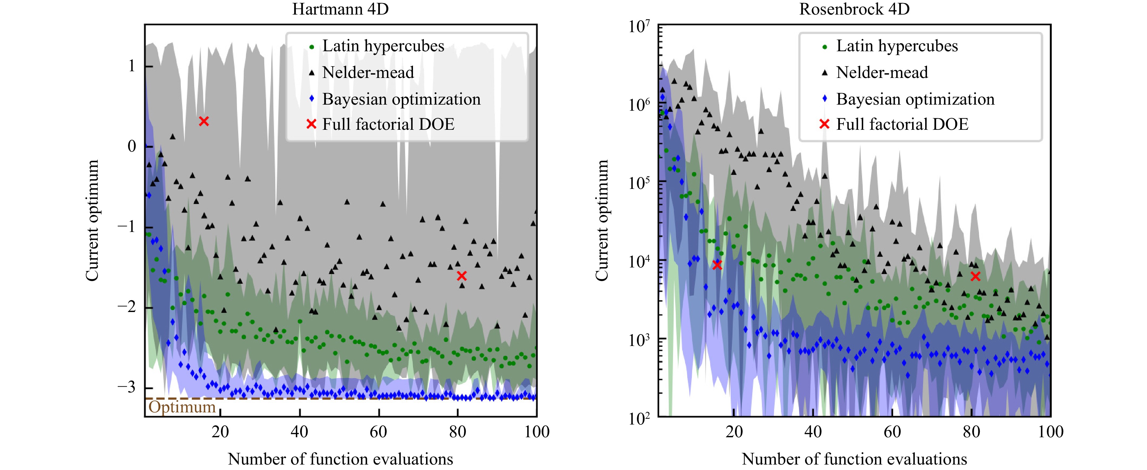
Fig. 1 Comparing various optimization techniques on two test functions, namely the Hartmann 4D and Rosenbrock functions. The optimization process is iterated ten times, and the displayed results represent the mean. The partially transparent uncertainty bands indicate the range between the maximum and minimum values obtained from the ten optimization runs. For the Hartmann 4D function, the optimal value is approximately −3.14, while for the Rosenbrock function, the optimum is at 0.
In both the Hartmann-4D and Rosenbrock functions, Bayesian optimization consistently identifies the smallest value and achieves the fastest convergence to this optimal point. Furthermore, Bayesian optimization yields minimal uncertainty regarding the discovered optimum, underscoring its generic applicability when seeking optima with a limited number of function evaluations.
-
The upcoming section illustrates and discusses the results obtained through Bayesian optimization applied to laser cutting, polishing, and welding. It is important to note that the expertise of laser process developers is solely utilized in establishing an appropriate cost function tailored to the particular process undergoing optimization. The process parameters as well as quality measures of the different laser processes are given in Table 4.
Parameter Explanation $A_P$ pore area fraction $C_N$ number of transverse cracks $C_t$ maximum depth of transverse cracks $\eta_P$ power fraction in core fiber $h_w$ height of weld top seam $h_b$ burr height $n_P$ number of laser pulses per burst $n_s$ number of scans $P$ laser power $p_{N_2}$ nitrogen gas pressure $R_z$ surface roughness $s$ cutting success $S_q$ surface roughness $t$ capillary depth $t_Z$ target capillary depth $U$ presence of undercuts $v$ welding speed/feed rate $z_f$ focal distance $z_N$ distance between gas nozzle and sample Table 4. Process parameters as well as quality measures of the applied laser processes.
-
The goal in Bayesian optimization of deep penetration laser welding was to quickly find process parameters that result in a specified weld depth $ {t_Z = 1.5\ \text{mm}} $ with minimal amount of defects and high welding speed. Thus, the chosen quality properties are the capillary depth $ t $, the pore area fraction $ A_P $, the number of transverse cracks $ C_N $ in the weld, the maximum depth of transverse cracks $ C_t $, the presence of undercuts $ {U \in \lbrace 0, 1 \rbrace} $, the height of the weld top seam $ h_w $, and the welding speed $ v $.
The process parameters that are varied are the laser power $ P $, the welding speed, the focal position $ z_f $ with respect to the sample surface, and the power fraction $ \eta_p $ in the core of the used BrightLine Weld fiber. Details of the technical setup and the evaluation of the welds are found in the methods section. The cost function is formulated to balance the maintenance of welding depth and the attainment of high welding speed as top priorities, while assigning comparatively lower weight to seam defects. Altogether, the employed cost function is designed as follows
$$ \begin{aligned} f_c({\boldsymbol{x}}) =\;& w_t |t ({\boldsymbol{x}}) -t_Z| + w_p A_P ({\boldsymbol{x}}) + w_n C_N ({\boldsymbol{x}}) \\& + w_c C_t ({\boldsymbol{x}}) + w_u U ({\boldsymbol{x}}) + w_h h_w ({\boldsymbol{x}}) \\ & + \frac{1}{2} \arctan \left( w_v \left( v_{\text{ref}} - v ({\boldsymbol{x}}) \right) \right) \\ {\boldsymbol{x}} =\;& \left(P, v, z_f, \eta_p \right) \\ w_t =\;& 2\ \text{mm}^{{-1}}\ \ w_p = 6.67\ \ w_n = 0.083 \\ \ \ \ \ w_c = \;&0.63\ \text{mm}^{{-1}} \ \ w_u = 0.16\ \ w_h = 0.25\ \text{mm}^{{-1}} \\ \ \ \ \ w_v =\;& 0.25\ \text{min/m} \ \ v_{\text{ref}} = 25\ \text{m/min} \end{aligned}$$ (9) Fig. 2 depicts the evaluated properties as well as the achieved values of the cost function during optimization. Initially, Sobol sequence parameters led to high cost function values due to improper process parameters causing heat conduction welding, indicated by small values of $ t $. As the Bayesian optimization starts from the ninth experiment the value of the cost function is clearly decreasing. The optimizer recognizes the necessary correlations of the process parameters to achieve the required capillary depth, approaching $ t_Z $ with ongoing optimization. Additionally, $ h_w $ decreases as the optimization proceeds. Internal defects are not a major problem throughout the optimization. From the chosen process parameters, a clear preference for relatively high feed rates is visible. The optimizer recognizes that this requires a high laser power to achieve the desired capillary depth. The best result for $ {n = 24} $ was achieved with $ {P = 8\ \text{kW}} $, $ {v = 30.7\ \text{m/min}} $, $ {z_f = 0.56\ \text{mm}} $, and $ {\eta_p = 0.49} $. No internal defects were visible and a capillary depth of $ {t = 1.54\ \text{mm}} $ was achieved. However, the weld seam shows clear undercuts, which were not critical in this application.
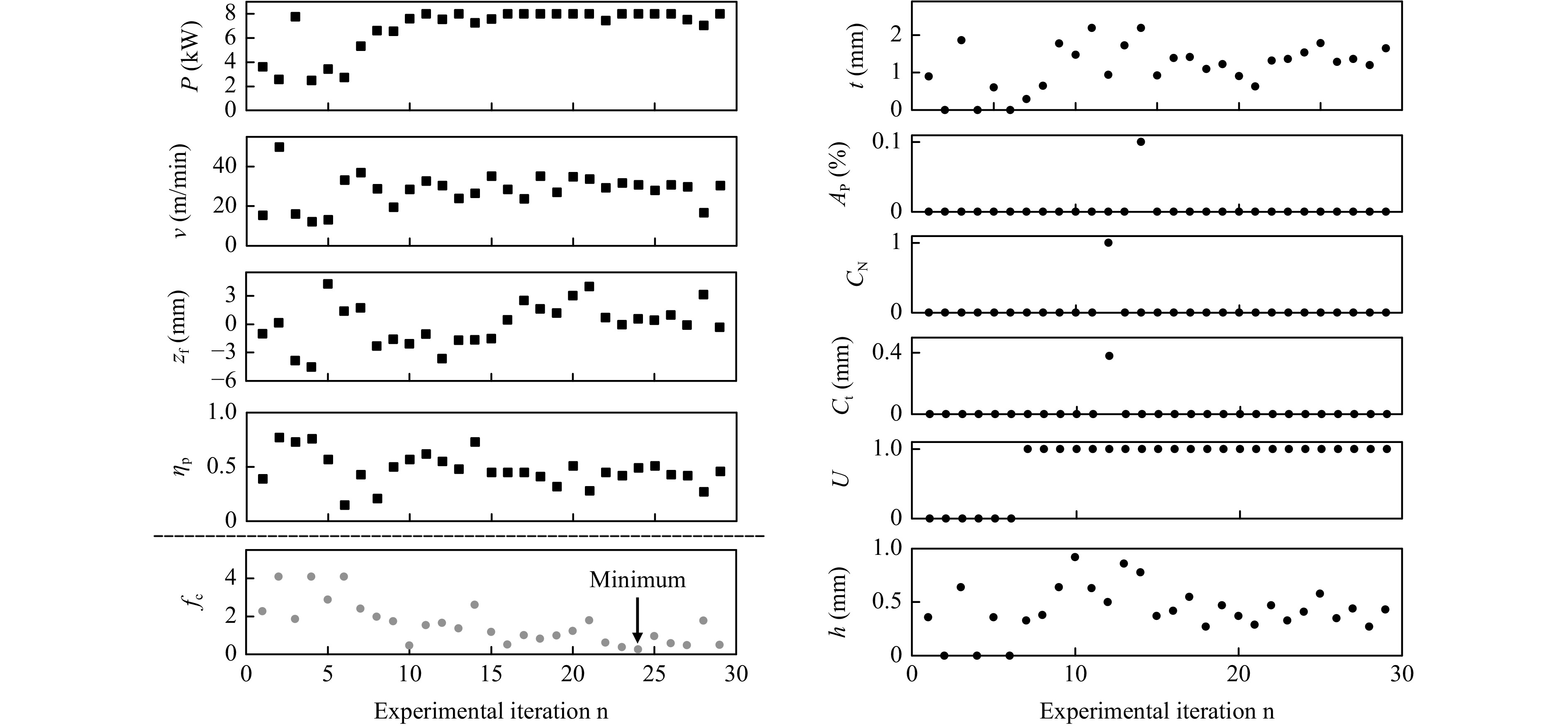
Fig. 2 Welding results. Evolution of process parameters, measured properties of the weld seam and value of the cost function during optimization of deep penetration laser welding.
-
For the laser polishing experiments, an ultrashort pulse laser was used in GHz burst mode to investigate the achievable reduction in roughness by laser polishing of 1.4301 stainless steel material starting from different initial surface conditions. The goal was for every initial roughness to find the polishing parameters that yield the lowest roughness after polishing. During optimization, we varied the average laser power $ P $, the number of laser pulses per burst $ n_p $, and the number of scans $ n_s $. Additional experimental parameters and detailed technical information about the laser system is provided in the methods section.
The evaluation focused solely on the resulting surface roughness $ S_{q,r} $, simplifying the formulation of the cost function as follows
$$ f_c(P, n_p, n_s) = w_q S_{q,r}(P, n_p, n_s);\ \ \ w_q = 1\ {{\mu}}{\text{m}}^{-1} $$ (10) Furthermore, we conducted an optimization run for various initial roughness values $ S_{q,i} $ ranging from $ {S_{q,i} = 8.7\ {{\mu}}{\text{m}}} $ to $ {S_{q,i} = 77\ {{\mu}}{\text{m}}} $. Details regarding the generation of $ S_{q,i} $ are provided in the methods section. To manage this extensive set of experiments, we limited the experimental iterations for a specific $ S_{q,i} $ to $ N = 15 $, with the first six iterations being part of the Sobol sequence.
Fig. 3 exemplary depicts the optimization processes for $ S_{q,i} = 50\ {{\mu}}{\text{m}} $, indicating a plateau reached after $ {n \geq 10} $ experimental iterations. A comparable behavior was observed for other investigated $ S_{q,i} $ values.
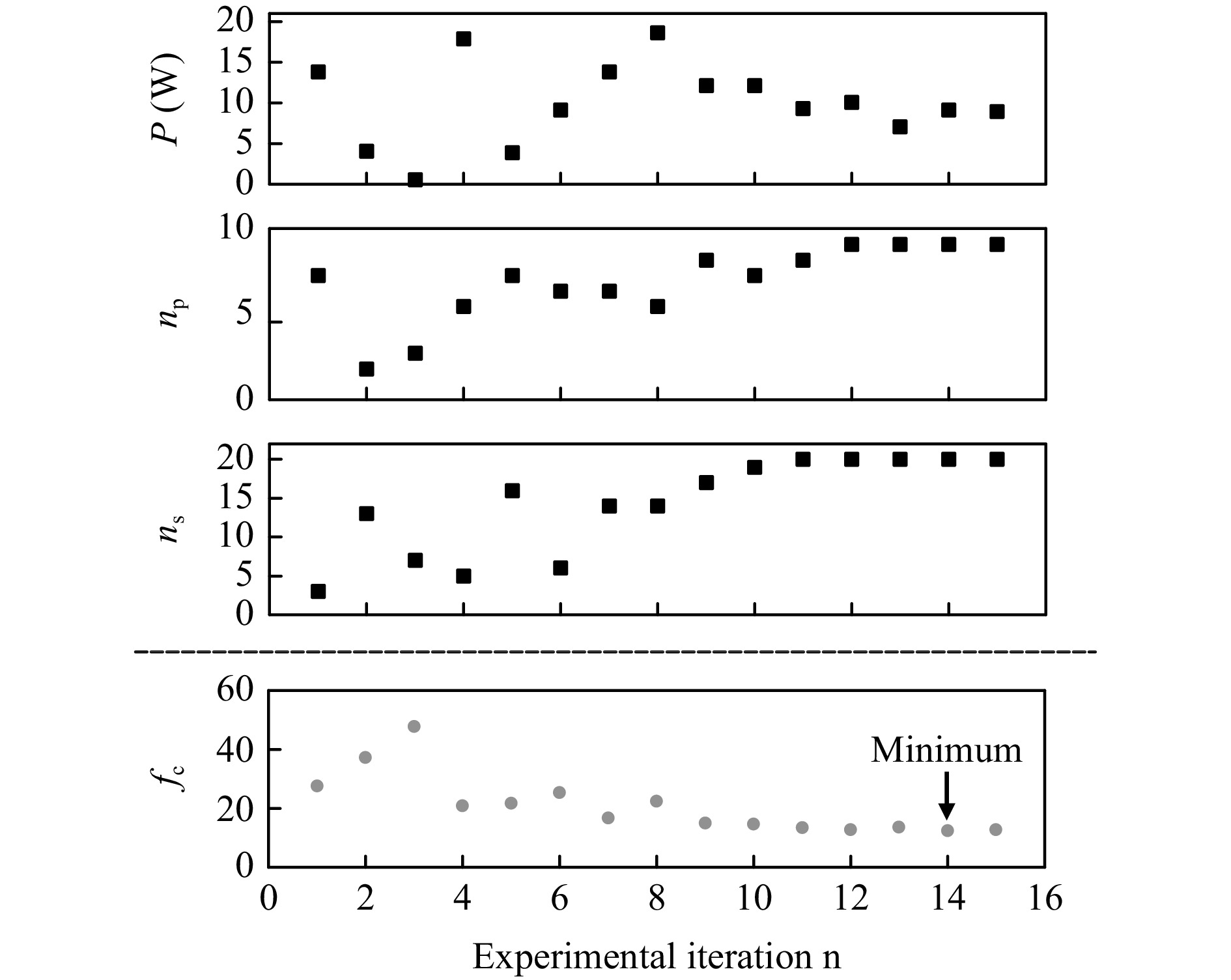
Fig. 3 Progress of the laser polishing iterations exemplary shown for the experiments with an initial roughness $S_{q,i}$ = 50 µm.
Fig. 4 compares the results of the best laser polishing processes obtained from Bayesian optimization for different $ S_{q,i} $ values. Remarkably, the polishing process achieved a reduction in surface roughness between 67% and 90% for all $ S_{q,i} $.
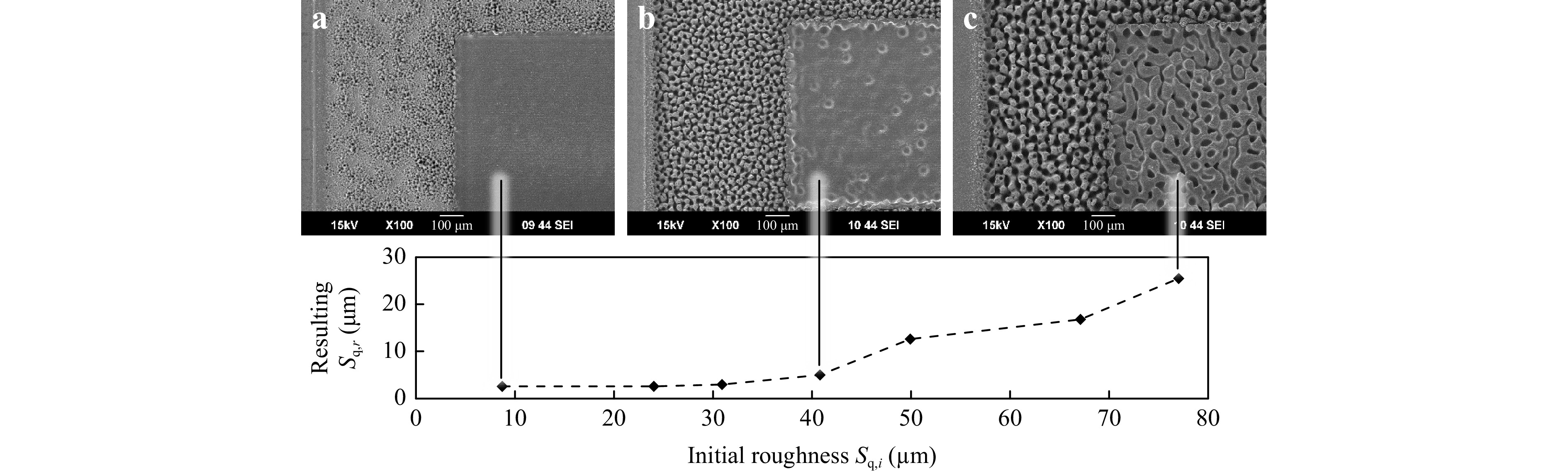
Fig. 4 Results for GHz laser polishing on different intial surface conditions. The scanning electron microsope images at a, b, and c show parts of the initial surface (left) and the polished surfaces (right).
The scanning electron microscope (SEM) images of the surfaces depict the initial rough surface and the polished areas. Adequate polishing results are achieved with no remnants of the initial surface structure visible up to an $ S_{q,i} \approx 40\ {{\mu}}{\text{m}} $. For $ S_{q,i} > 40\ {{\mu}}{\text{m}} $, melt formation is still present and the initial spikes are smoothed, but dimples and portions of the initial surface structure remain on the surface. Consequently, the minimal achievable roughness increases with $ S_{q,i} > 40\ {{\mu}}{\text{m}} $.
The allowable process time for polishing was in this study limited by setting the upper search space boundary for the number of scans $ n_{s,max} = 20 $, see methods section. However, the progress of the BO experiments suggests that this boundary is a limiting factor for the achievable result $ S_{q,r} $ beyond $ S_{q,i} > 40\ {{\mu}}{\text{m}} $ with the given setup.
Another finding is, that the resulting optimal peak fluence per burst pulse for all seven BO experiments ranges from 1.8 J/cm2 to 3.8 J/cm2. This is well above the ablation threshold of 0.075 J/cm2 27, and three orders of magnitude above the fluence per burst pulse of 2 mJ/cm2 used for polishing 1.4301 material in Ref. 28. The presence of a particle seam surrounding the polishing areas supports the assumption, that the optimized parameters do not lead to conventional melting-based polishing processes. Instead, ablative material removal appears to be partially harnessed to achieve effective roughness reduction within specified constraints.
-
The effectiveness of Bayesian optimization was assessed for laser cutting of $ 5\ \text{mm} $ stainless steel sheets. Detailed experimental procedures can be found in the methods section.
The varied process parameters encompassed the laser power $ P $, feed rate $ v $, nitrogen gas pressure $ p_{N_2} $, distance of the gas nozzle to the sample's top surface $ z_{n} $, and the focal distance with respect to the gas nozzle position $ z_f $. The methods section outlines the permissible range of technical variations for these parameters.
The considered quality properties encompass the cutting success $ {s \in \lbrace 0, 1 \rbrace} $, where $ {s = 1} $ signifies a successful cut. In the case of a successful cut, the other quality factors are the burr height $ h_b $, feed rate $ v $, and the roughness $ R_z $. The methods section summarizes the methods for determining these quantities.
In defining the cost function, our primary focus is on ensuring cutting success, with burr height taking precedence over roughness and feed rate, which are considered nearly equal, resulting in
$$ \begin{array}{l} f_c({\boldsymbol{x}}) = \left\{ {\begin{array}{*{20}{l}} {5 \times 10^3; }&{s = 0 }\\ {w_h h_b ({\boldsymbol{x}}) - w_v v ({\boldsymbol{x}}) + w_r R_z ({\boldsymbol{x}}); }&{s = 1 } \end{array}} \right.\\ \ \ \ \ \ {\boldsymbol{x}} = (P, v, p_{N_2}, z_n, z_f) \\ \ \ \ w_h = 50\ \text{mm}^{-1}; \ \ \ w_v = 5 \times 10^{-4}\ \text{min}/\text{mm}; \\ \ \ \ w_r = 10\ \text{mm}^{-1} \end{array}$$ (11) Cutting success is highest prioritized by introducing a penalty of $ {5 \times 10^3} $ to $ f_c $ when the cut fails. The weights signify prioritization of burr height over feed rate and roughness, under the expected conditions where $ h_b \in [0, 5\ \text{mm}] $, $ {v \in[0, 5 \times 10^3\ \text{mm}/\text{min}]} $, and $ {R_z \in [0, 0.5\ \text{mm}]} $.
The results of the optimization process are depicted in Fig. 5. The minimum of the cost function was achieved after $ {n = 31} $ iterations, resulting in $ {h_b = 0.04\ \text{mm}} $, $ {v = 1351\ \text{mm/min}} $, and $ {R_z = 0.37\ \text{mm}} $. The initial ten iterations were part of the Sobol sequence. Beyond $ {n = 31} $, the optimization entered a plateau, leading to termination after $ {N = 103} $ iterations.
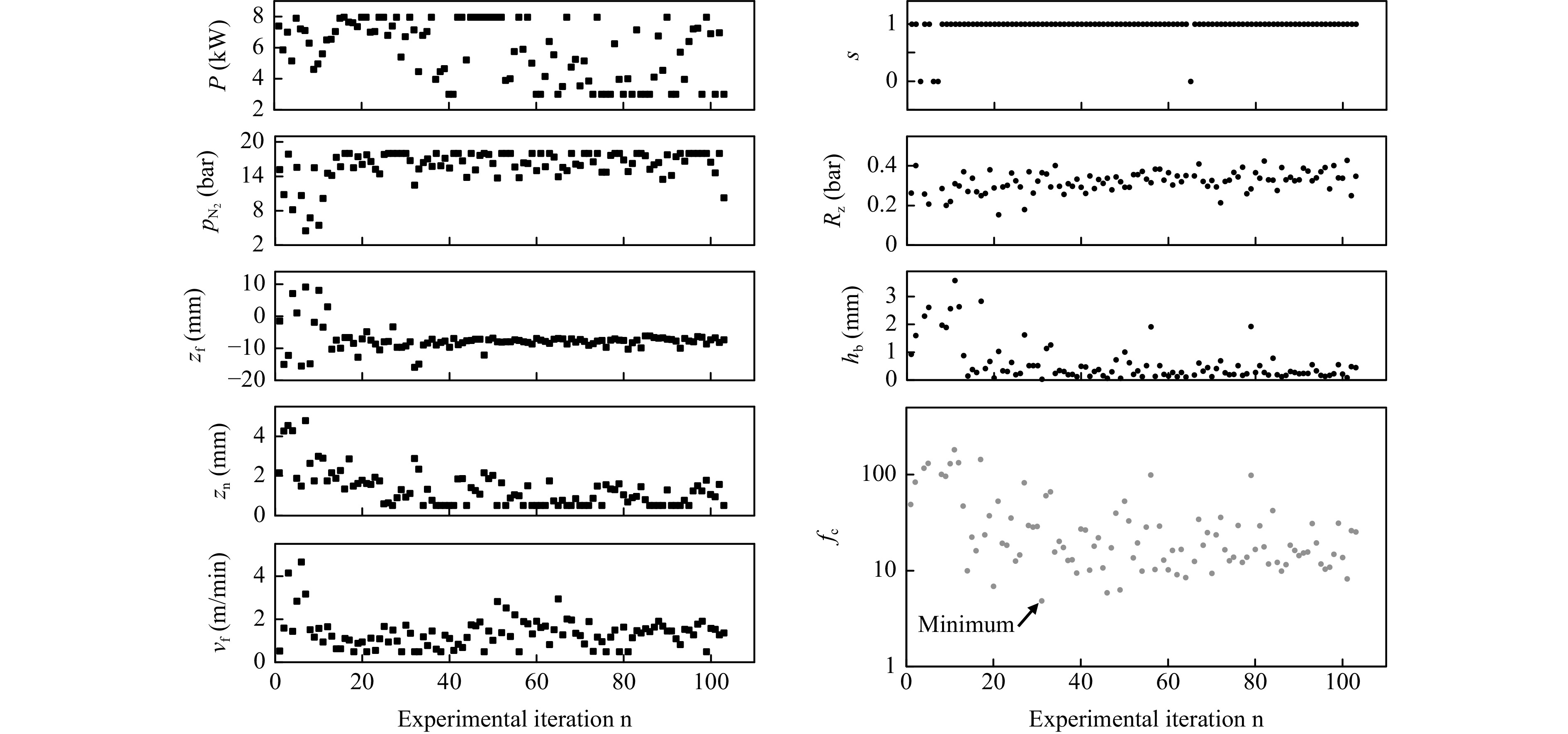
Fig. 5 Cutting results. Process parameters and cost function for laser cutting.
A comparison of the weighted cost defining properties $ {w_h h_b} $, $ {w_v v} $, and $ {w_r R_z} $ in Fig. 6 reveals that the optimization is primarily influenced by $ h_b $, aligned with the prioritization expressed by $ f_c $. The optimization process effectively reduces $ h_b $, besides some peaks due to exploration. However, it appears that the weights assigned to $ v $ and $ R_z $ may be relatively low, causing these variables to exhibit minimal impact. Moreover, the minor emphasis on $ v $ results in lower values when compared to those reported in the literature29.
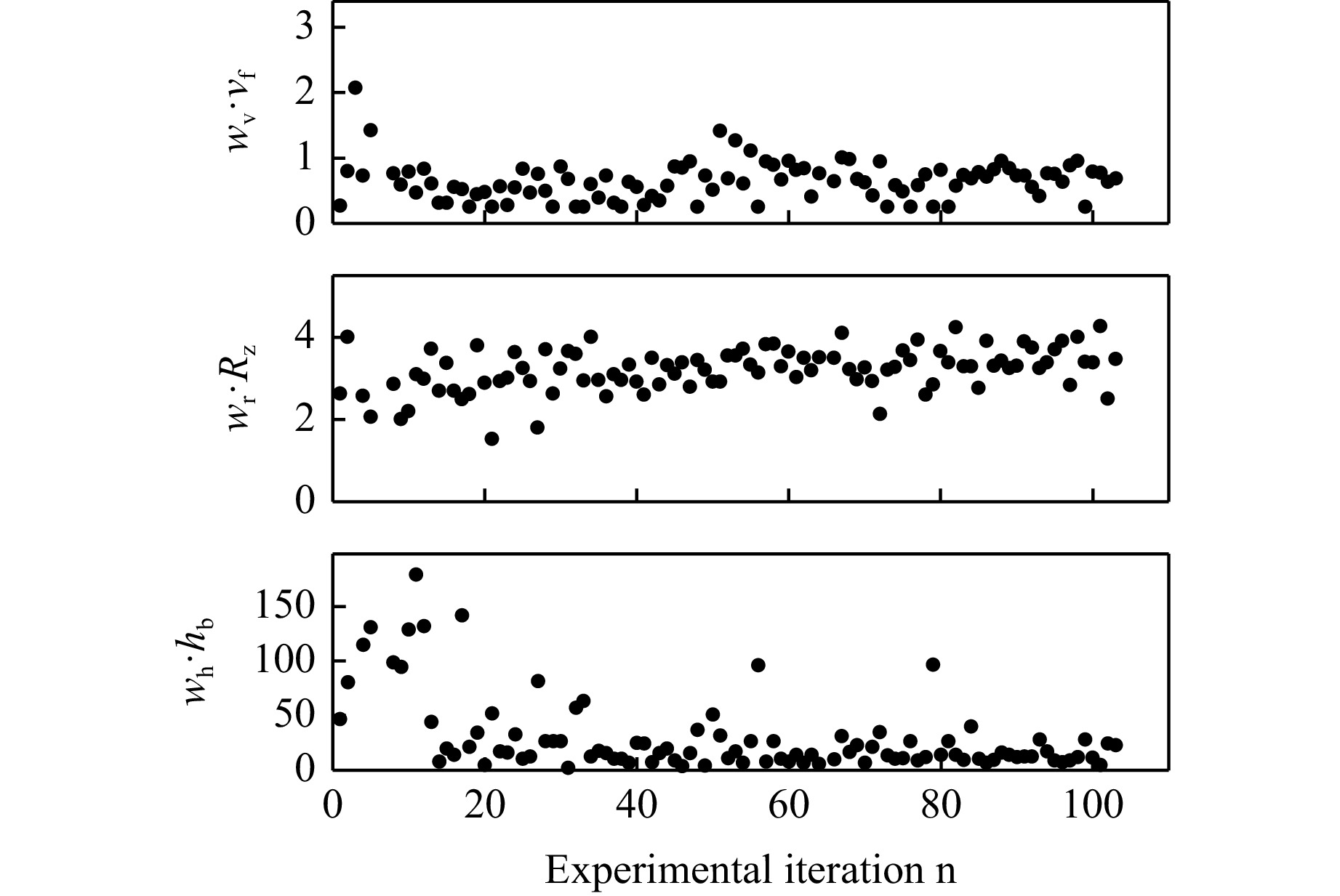
Fig. 6 Cutting results. Weighted inputs of feed rate, roughness, and burr height into the cost function.
Furthermore, the definition of $ f_c $ in Eq. 11 exhibits unsteady behavior concerning $ s $. Utilizing the Ax default squared exponential kernel for the optimization might be inconvenient, as it is best suited for approximating smooth and steady functions14. In such cases, Matérn kernels could be a more suitable choice14. Alternatively, instead of using $ s $, one could consider employing a continuous property, such as cut depth, which must precisely match the sample thickness.
-
In conclusion, this study demonstrates the practical application of Bayesian optimization in optimizing various laser processes such as welding, polishing, and cutting. Our findings emphasize the readiness of this optimization technique for adoption by laser process developers in real-world scenarios. Utilizing the user-friendly Ax framework, our experiments showcased the potential of optimizing laser processes with only a few tens of experimental iterations. However, it is crucial to highlight the significance of expert knowledge in formulating accurate cost functions related to laser processes. Additionally, a basic understanding of the underlying mathematical aspects of Bayesian optimization, including the selection of appropriate kernels, is essential for satisfactory results.
In the case of laser welding the Bayesian optimizer allowed to quickly find process parameters that resulted in a weld with the desired seam depth and no internal defects without requiring prior knowledge. These parameters correspond to those recommended by experts. The optimization could be carried out in less than five hours and is therefore economically attractive. The fast analysis of the samples and updating the model after each experiment significantly reduces the required time.
In the context of laser polishing, we have successfully identified effective polishing processes for surfaces with high initial roughness values ranging from $ {S_{q,i} = 8.7\ {{\mu}}{\text{m}}} $ to $ {S_{q,i} \approx 40\ {{\mu}}{\text{m}}} $. For all $ {S_{q,i}} $ the optimization found a polishing process that improves the roughness by more than $ 67\ \% $. Notably, this was achieved through a remarkably low number of only 15 experimental iterations. Furthermore, the optimization outcome is not a pure melt-based polishing process, which is in contrast to the commonly reported GHz polishing methods28. It is reasonable to assume that such a conventional polishing approach would not have been successful on the highly rough surfaces tested in our study.
In laser cutting, we conducted an optimization process that prioritized cutting success, burr height, feed rate, and roughness, in that order. After conducting 31 experiments, we determined the best process based on a cost function that reflected this prioritization. In case of cutting success, the optimization was primarily influenced by burr height, aligning with our prioritization criteria. However, it appears that the weight assigned to the feed rate was potentially too low. Consequently, the optimized process is notably slower compared to the extreme feed rates reported in the literature.
-
In this section the detailed experimental setups and evaluation methods are described for the three investigated processes of laser welding, polishing and cutting.
-
A solid state cw laser with a wavelength of $ {\lambda = 1030\ \text{nm}} $ and a maximum power of $ {P = 8\ \text{kW}} $ in combination with a multi core BrightLine Weld fiber from TRUMPF was used for the welding experiments. The focal length of the collimating lens was 200 mm while the focal length of the focusing lens was 280 mm. With core and ring fiber diameters of 100 µm and 400 µm the beam waist diameter is 140 µm and 560 µm, respectively. Bead-on-plate welding of 80 mm long welds was performed on 4 mm thick samples of AA5754 aluminum. The experiments were conducted inside a high-speed X-ray diagnostics system to be able to investigate the capillary and internal defects within the weld seam. The X-ray system has been described in literature in detail30. The welding process was recorded at a frame rate of 500 Hz with an acceleration voltage of the X-ray tube of 50 kV and a tube power of 75 W.
For the welding experiments it was of interest to find process parameters that result in a specified weld depth with minimal defects and high welding speed. The weld depth directly determines the joining area and thus the mechanical strength, but can only be determined by metallographic sections. To perform the evaluation promptly after the welding process, the capillary depth $ t $ is determined instead. Previous studies have shown the correlation between the depth of the capillary and the resulting depth of the weld seam in case of deep penetration laser welding31, 32. To determine the capillary depth the X-ray images of the sample captured during the welding process were averaged. The depth of the capillary was measured using a fixed threshold of the grayscale values.
Welding, particularly in aluminum alloys, is prone to internal defects like pores and cracks, which can significantly comprise weld quality33. In order to quickly examine the internal defects, the welded samples were again analyzed with the X-ray tube after the welding process. Since the defects have already solidified, they are visible in multiple images. As a result, it is possible to overlay and average the images to reduce noise. Through this averaging both pores and transversal cracks are visible in the images, compare Fig. 7a. By binarizing the image with a fixed threshold value, the pores and cracks can be distinguished from the surrounding bulk material. The circularity of the detected objects allows further differentiation between pores and transverse cracks, as can be seen in Fig. 7b as red and blue marks. Compared to the test weld in Fig. 7a, no internal defects can be seen in the X-ray image for the optimum parameters from Fig. 2.
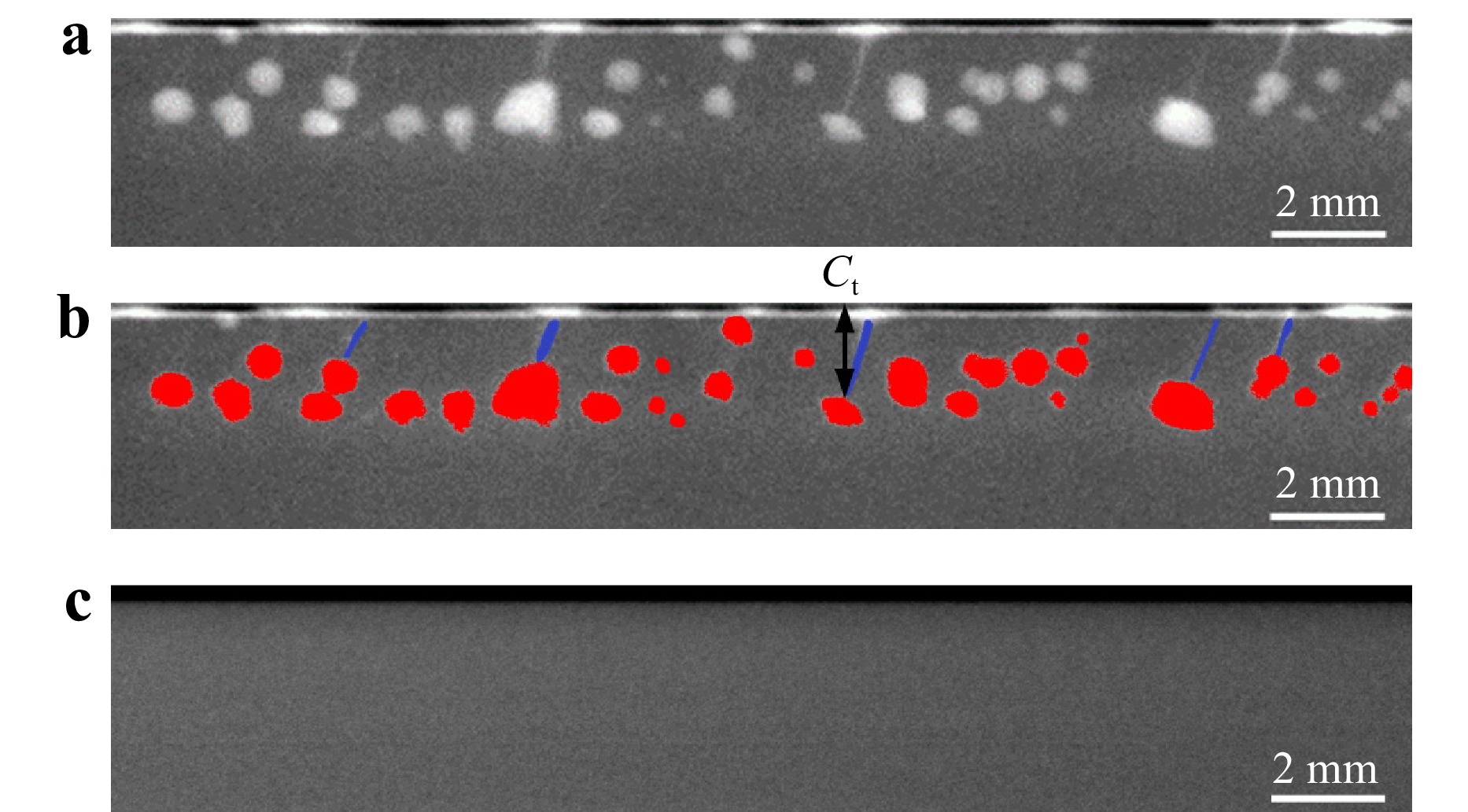
Fig. 7 Welding results. Analysis of the X-ray images of the weld seams: a superimposed image of a test weld seam after the welding process, b marked pore area fraction (red), cracks (blue) and maximum depth of cracks $ C_t$, c superimposed image for the best welding experiment ($ n=24$).
To quantify the defects a 50 mm long area was selected in the superimposed X-ray image, excluding the start and end of the weld. The depth of the area was set to the capillary depth. The share of the pore area inside this area can be used to quantify the amount of pores and is referred to as the pore area fraction $ A_P $. Transverse cracks were characterized by their number $ C_N $ within the weld seam and the maximum depth $ C_t $ of the deepest crack. To detect humping the maximum height $ h_w $ of the weld top bead was measured with a caliper gauge, excluding the start of the weld and the end crater.
To prevent the optimizer from suggesting inappropriate process parameters, the possible range was limited for each parameter. Therefore, the welding speed $ v $ was limited to a range between 3 and 50 m/min and the focal distance to $ {z_f = \pm5\ \text{mm}} $. The lower limit of the laser power $ P $ was restricted to values above 1 kW to facilitate deep penetration welding. The upper limit was limited to a speed-dependent value for welding speeds below 10 m/min to prevent damage to the setup. For higher welding speeds the laser power is limited by the available maximum power of 8 kW of the laser.
-
For laser polishing, an ultrashort pulse laser was used in GHz burst mode. The goal was to investigate the achievable reduction in roughness on different initial surface conditions on 1.4301 stainless steel material. The initial roughness was produced in preparation with laser ablation processes without bursts using high peak fluences from 5.6 J/cm2 to 29 J/cm2, which yield roughness values $ S_{q,i} $ ranging from 8.7 µm to 77 µm.
The polishing laser Carbide CB3-80 (Light Conversion, Lithuania) operated at $ \lambda $ = 1030 nm. The beam was circular polarized, configured for 190 fs pulse duration at a pulse repetition rate of 50 kHz and focused to a spot on the surface of 50 µm. For beam steering a 2d galvanometer scanner was used with an f-theta lens of 163 mm focal length. The feed was constant at 500 mm/s with a 10 µm hatching distance. The variable parameters for optimization were average laser power between 0.15 W and 18.6 W, the number of pulses per burst packet from 1 to 10 with a delay of 440 ps and the number of scans from 1 to 20.
There are multiple metrics to quantify the surface roughness of a specimen, which can be separated into profile and areal measurements. In this case the common areal roughness value Sq in µm provided a direct cost value, see Eq. 10. It was measured using an inline coaxial optical coherence tomography sensor Chrocodile2 (Precitec Optronik GmbH, Germany)34. A best fit tilted plane was subtracted from the raw topography. By focusing through the same optics the OCT’s minimum focus diameter is limited and the measured roughness values have to be interpreted mainly qualitatively. However, the OCT technology has the advantage of being fully integratable into the ablation systems to measure the process result without movement of the sample or change of the processing head. This saves time and labor and enables a complete automation of such optimization tasks.
-
For laser cutting a solid state cw laser with a wavelength of $ \lambda = 1030\ \text{nm} $ and an adjustable maximum power of $ P = 8\ \text{kW} $ with a transport fiber with a core diameter of 100 µm was used. The laser beam was focused to the work piece with a Pro Cutter 2 cutting head from Precitec with a collimating lens with 100 mm focal length while the focal length of the focusing lens was 150 mm, leading to a focus diameter of about 150 µm. The cutting nozzle had a nozzle diameter of 3 mm. As cutting gas Nitrogen with purity level 5.0 was used. For the optimization these parameters were constant. Varied process parameters were the average power of the laser between 3 kW to 8 kW, the gas pressure $ p_{N_2} $ between 3 bar to 18 bar, the feed rate $ v $ between 0.5 m/min to 8 m/min, the focal position between −16 mm to 10 mm. The nozzle distance to the surface was varied between 0.5 mm to 5 mm. The material used was 5 mm thick stainless steel 1.4301. The target parameters for the optimization were the roughness $ R_z $, feed rate $ v $ and the maximum burr heigth $ h_b $. Therefore, a cut was made over a length of 60 mm per experiment. For the evaluation of the cut quality, the cut edge was measured in the range from 20 mm after the start of the cut to a length of 40 mm with a surfacecCONTROL 3D 3500 sensor to determine the roughness $ R_z $ according to the ISO 25178 standard and the burr height $ h_b $.
-
The authors would like to thank the Ministry of Science, Research and Arts of the Federal State of Baden-Württemberg for the financial support of the projects within the InnovationsCampus Mobilität der Zukunft as well as for the sustainability support of the projects of the Exzellenzinitiative II. The authors would like to thank Precitec Optronik GmbH (Germany) for providing the OCT sensor Chrocodile2. The authors would like to thank Light Conversion (Lithuania) for providing the Carbide CB3-80 laser. The Laser beam source TruDisk8001 (DFG object number: 625617) was funded by the Deutsche Forschungsgemeinschaft (DFG, German Research Foundation) – INST 41/990-1 FUGG.
Laser material processing optimization using bayesian optimization: a generic tool
-
Tobias Menold1, *, ,
 ,
, - Volkher Onuseit1,
- Matthias Buser1,
- Michael Haas1, 2,
- Nico Bär1,
- Andreas Michalowski1
- Light: Advanced Manufacturing 5, Article number: 32 (2024)
- Received: 02 November 2023
- Revised: 29 May 2024
- Accepted: 30 May 2024 Published online: 23 September 2024
doi: https://doi.org/10.37188/lam.2024.032
Abstract: Optimizing laser processes is historically challenging, requiring extensive and costly experimentation. To solve this issue, we apply Bayesian optimization for process parameter optimization to laser cutting, welding, and polishing. We demonstrate how readily available Bayesian optimization frameworks enable efficient optimization of laser processes with only modest expert knowledge. Case studies on laser cutting, welding, and polishing highlight its adaptability to real-world manufacturing scenarios. Moreover, the examples emphasize that with suitable cost functions and boundaries an acceptable optimization result can be achieved after a reasonable number of experiments.
Research Summary
Laser Material Processing Optimization using Bayesian Optimization
Scientists from the Institut für Strahlwerkzeuge (IFSW) at the University of Stuttgart applied Bayesian optimization for process parameter optimization in laser cutting, welding, and polishing. The IFSW scientists demonstrated how readily available Bayesian optimization frameworks enable efficient optimization of laser processes with only modest expert knowledge. Case studies on laser cutting, welding, and polishing highlight its adaptability to real-world manufacturing scenarios. Moreover, the examples emphasize that with suitable cost functions and boundaries, an acceptable optimization result can be achieved after a reasonable number of experiments.
Rights and permissions
Open Access This article is licensed under a Creative Commons Attribution 4.0 International License, which permits use, sharing, adaptation, distribution and reproduction in any medium or format, as long as you give appropriate credit to the original author(s) and the source, provide a link to the Creative Commons license, and indicate if changes were made. The images or other third party material in this article are included in the article′s Creative Commons license, unless indicated otherwise in a credit line to the material. If material is not included in the article′s Creative Commons license and your intended use is not permitted by statutory regulation or exceeds the permitted use, you will need to obtain permission directly from the copyright holder. To view a copy of this license, visit http://creativecommons.org/licenses/by/4.0/.

 DownLoad: