


HTML
-
Intelligent optical manufacturing is a cross-disciplinary integration of advanced manufacturing, precision control, materials, and artificial intelligence. The potential to achieve enhanced machining quality by implementing robot-based precision motion control has been demonstrated1. Nevertheless, as optical components evolve from simple forms to spatially asymmetric multi-degree-of-freedom complex surfaces, machining precision evolves to the nano-level or even higher; accordingly, the difficulty in achieving highly consistent fine optical manufacturing increases significantly2,3. The material properties of the optical components make considering the control performance of both the operating motion information and contact force necessary. Even small position deviations or force fluctuations can lead to optical surface deviations, further affecting the imaging quality and transmission efficiency of optical systems.
Constant force control has been introduced into robot-assisted polishing technology to achieve uniform polishing of complex surface. By using passive or active compliance control, a constant contact force with small fluctuations in relation to the geometrical profile of the optical component has been achieved4,5. Nevertheless, the manipulated force may vary with specific processing tasks in complex optical manufacturing processes, making robot-based control substantially complicated. In Ref. 6, the contact force was planned and dynamically modified based on the material removal model along the grinding tool path, and a higher and more uniform contour accuracy was achieved for curved surfaces compared to constant force control. Moreover, as indicated by comparison of the effects of manual operation and robotic grinding in Ref. 7, although the processing efficiency of robotic grinding has increased dramatically, its consistency remains inferior to that of manual operation. This may be because human hands are more perceptive to changes in haptic (position and force) information, and their manipulation experience is difficult to be completely transferred via only programming. In practical optical processing, precision operations rely heavily on the expert manufacturing experience. However, the need for consistent quality, efficiency, and safety necessitates robot-based solutions. Consequently, the intelligent acquisition and reproduction of haptic information from experts’ manipulations to robots has received considerable attention in recent years8,9.
Skill learning technologies can factually and comprehensively acquire manipulation characteristics of experts and precisely reproduce them on robots10,11, realising human skill transfer. In this regard, learning from demonstration (LfD) and motion copying are two typical methods. LfD entails the extraction of the rules of human operation via drag-based or wearable-equipment-based demonstrations or demonstration videos. Thereafter, motion planning models are constructed to reproduce and generalise the manipulation12,13. This method provides intelligent sensing, decision-making, and learning capabilities for complex manipulation skills. However, the human-robot interaction force and contact force from the environment are prone to coupling and difficult to identify14. Motion copying is a relatively direct motion reproduction method. In general, a motion-copying system (MCS) consists of a motion-saving subsystem (MSSS) and motion-reproducing subsystem (MRSS)15. The MSSS saves the operator’s haptic information in a motion database that serves as the virtual master motion, and the stored motion is reproduced repeatedly on the slave side of the MRSS. On the basis of bilateral control, the operator can directly manipulate conventional processing equipment in a more conventional manner, and the action and reaction forces between the manipulator and the environment are separated to improve the accuracy of force detection16. This approach has been implemented for applications such as calligraphy and grasping robots. However, it remains underutilised in the field of optical manufacturing.
The manipulation characteristics of optical manufacturing pose challenges with regard to the direct application of motion copying. First, the location of the manipulated object changes during repetitive operations. For example, in optical cutting or grinding in subtractive manufacturing, the position of the optical surface in contact with the manufacturing robot changes with the removal of unnecessary materials from the workpiece17. Accordingly, the machining strategy must be intelligently adjusted to accommodate the location changes of the object in each operation, thereby avoiding manufacturing motion errors that change the processing trajectory and degrade the optical surface quality18. To solve this issue concerning the location change of the objects, improved strategies for motion copying have been proposed. In Ref. 19, a high-stiffness MRSS and a highly adaptive MRSS were realised to accommodate geometric position relation changes between the manipulator and contact surface or additional force. However, this approach necessitates prior knowledge of the environmental changes. A velocity-force hybrid control that does not rely on any prior knowledge was designed for the MRSS20; however, the reproduction consistency with the location change of the object is limited. An online motion modification method was proposed, and the manipulation of the operator was added to the MRSS with weights to improve flexibility in task completion21. However, the consistency of multiple processing steps is no longer guaranteed. Generally, these methods cannot achieve motion replication with high repetition consistency under the condition of unknown location changes.
Furthermore, the manipulating force is typically not constant, and the manipulation is switched back and forth between free and constrained spaces, which is more challenging to replicate than a constant force. Reliable force measurements are a prerequisite for precise force control. Typically, force sensors are mounted at the end effectors of the robots and can measure the contact force between the robot and an uncertain workpiece environment in real time22. The force-sensor-based method is marked by its operational simplicity but requires additional mounted spatial space and cost. The reaction force observer (RFOB) is a force-sensorless estimation method for the contact force based on a disturbance observer. It avoids the limitation of sensor placement and can obtain a higher force control bandwidth23,24. However, the performances of RFOBs with low-pass filters are limited when the contact force changes abruptly. A sliding-mode-assisted disturbance observer with an adaptive-switching gain was proposed to improve the robustness against changing disturbances25. This method can be directly transferred into RFOBs; however, its ‘instantaneous increasing’ adjustment strategy may likely lead to input saturation if not appropriately set.
In general, given the precise motion transfer requirements for complex optical manufacturing, existing methods cannot solve the problem of high-consistency motion copy with the unknown location change of object, as well as precise force sensing and control under frequent motion space switching. Therefore, these current approaches cannot be directly implemented in expert motion copy and reproduction for optical manufacturing. To address these issues, this study investigated a novel motion-copying strategy. The main contributions of this study are as follows:
1. In line with the actual requirements of optical manufacturing, a motion-copying method with symbol sequence-based phase switch control (SSPSC) was devised. The completed manipulation is decomposed, symbolised, rearranged, and reproduced according to manufacturing characteristics. The switching stability of the SSPSC was examined. The proposed method accomplishes the transfer and reproduction of expert skills with high consistency and adaptability to location uncertainties.
2. A new adaptive sliding-mode-assisted reaction force observer (ASMARFOB) was devised. The dual-layer adaptive law with adaptive sliding manifold and switching gain was designed, yielding a remarkable enhancement in the estimation precision of the manipulated force with wider bandwidth. The uniformly ultimate boundedness (UUB) of the method is guaranteed.
-
The underlying concept of the proposed motion-copying scheme for intelligent optical manufacturing is illustrated in Fig.1. The motion-copying scheme entails MSSS and MRSS procedures. During MSSS, a technician manipulates the master side, and the slave side acts on the optical component in synchronisation via bilateral control. The operating information from the master side is automatically stored in a motion database in accordance with the motion phase. During MRSS, the stored manipulation is completely reproduced, and the motion phases are rearranged in real time according to the change in the initial location of the optical component. Thus, the manipulated optical manufacturing skills are reproduced.
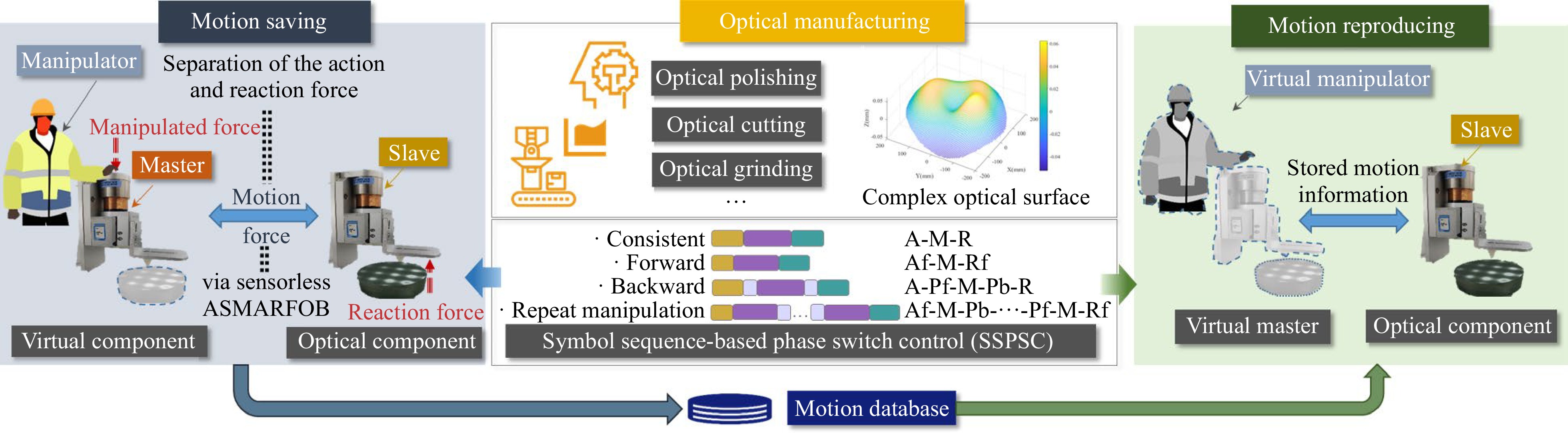
Fig. 1 Concept of the proposed motion-copying scheme
For design simplicity, a single-degree-of-freedom MCS was considered in this study; this can be easily extended to multi-degree-of-freedom systems. Without loss of generality, the master and slave actuators in MCS are modelled as
$$ \begin{array}{*{20}{l}} J_{i}\ddot{x}_{i}^{(j)}+B_i\dot{x}_{i}^{(j)}=u_{ri}^{(j)}-f_{i}^{(j)}+d_{i}^{(j)} \end{array} $$ (1) where $ i= m,s$ represents the master or slave, $ j=S,R $ represents MSSS or MRSS. $ \dot{x}_{i}^{(j)} $, and $ \ddot{x}_{i}^{(j)} $ denote velocity, and acceleration of actuators, respectively; $ J_i >0$ and $ B_i > 0 $ are the inertia mass and damping of the actuator in MCS, respectively; $ u_{ri}^{(j)} $ is the control input; $ f_{m}^{(j)} $ represents the force of operator exerted on the master actuator, and $ f_{s}^{(j)} $ represents environment force exerted on the slave actuator. $ d_{i}^{(j)} $ is the internal disturbance of the actuator, including friction and torque ripples, etc.
Considering the model uncertainties of the MCS, its nominal dynamics of MCS can be expressed as
$$ \begin{array}{*{20}{l}} J_{ni}\ddot{x}_{i}^{(j)}+B_{ni}\dot{x}_{i}^{(j)}=u_{ri}^{(j)}-f_{i}^{(j)}+d_{ti}^{(j)} \end{array} $$ (2) where $ J_{ni}=J_{i}-\bigtriangleup J_{i} $ and $ B_{ni}=B_{i}-\bigtriangleup B_{i} $ denote the nominal inertial mass and damping of the actuator in MCS, respectively. $ \bigtriangleup J_{i} $, and $ \bigtriangleup B_{i} $ represent the uncertain parts of $ J_{i} $ and $ B_{i} $, respectively. Further, $ d_{ti}^{(j)}=d_{i}^{(j)}-\bigtriangleup J_{i}\ddot{x}_{i}^{(j)}-\bigtriangleup B_{i}\dot{x}_{i}^{(j)} $.
By ensuring that $ d_{ti}^{(j)} $ is compensated by $ u_{ti}^{(j)} $ via disturbance compensation methods, Eq. 2 can be further transformed into Eq. 3.
$$ \begin{array}{*{20}{l}} J_{ni}\ddot{x}_{i}^{(j)}+B_{ni}\dot{x}_{i}^{(j)}=u_{i}^{(j)}- f_{i}^{(j)}-\varsigma_{i}^{(j)} \end{array} $$ (3) where $ u_{ri}^{(j)}=u_{i}^{(j)}-u_{ti}^{(j)} $; and $ \varsigma_{i}^{(j)}=u_{ti}^{(j)}-d_{ti}^{(j)} $ denote the disturbance compensation residuals. $ J_{nm}=J_{ns}=J_{n} $, and $ B_{nm}=B_{ns}=B_{n} $ for the same master and slave actuators.
Assumption 1: There exists an upper bound of $ \varsigma_{i}^{(j)} $, satisfying $ |\varsigma_{i}^{(j)}|\leq \bar{\varsigma}_{i}^{(j)} $ and $ \varsigma_{i}^{(j)}\to 0 $ with proper compensation method26.
Considering the stiffness and damping characteristics in the contact environment, the Kelvin-Voigt contact model is used to represent the environmental force $ f_{s}^{(j)} $ when the MCS is in contact with the manipulated object.
$$ \begin{array}{*{20}{l}} f_{s}^{(j)} = k_ex_s^{(j)}+b_e\dot{x}_s^{(j)} \end{array} $$ (4) where $ k_e $, and $ b_e $ are the stiffness and damping coefficients, respectively, of the manipulated object. For intelligent optical manufacturing, a manipulated object is typically composed of metallic materials, which can be considered stiff and $ k_e\gg b_e $.
In practical experiments, $ f_{i}^{(j)} $ depends on the action and reaction forces between the operator and manipulated object. Consequently, it can be considered to change slowly and continuously as compared to the system state in every sampling period. Therefore, the following assumption can be made:
Assumption 2: $ f_{i}^{(j)} $ and its time derivative $ \dot f_{i}^{(j)} $ are continuous, and $ \dot f_{i}^{(j)} $ is a bounded signal from the perspective of practical engineering although it is unknown27.
The goal of MCS for intelligent optical manufacturing is to accurately reproduce the manipulation force during the contact phase, regardless of the changes in the initial location of the manipulated object.
-
To replicate the manipulating characteristics of the experienced technician, a bilateral control strategy is employed in the MSSS, as depicted in Fig. 2a. The manipulator operates the master actuator and completes manipulations. Using a position–force bilateral controller, the control signal is transmitted to the slave actuator, and manufacturing manipulation is executed on the optical component. All motion data from the master side are saved in a motion database. Good transparency (position tracking and force feedback) is ensured throughout the manipulation process.
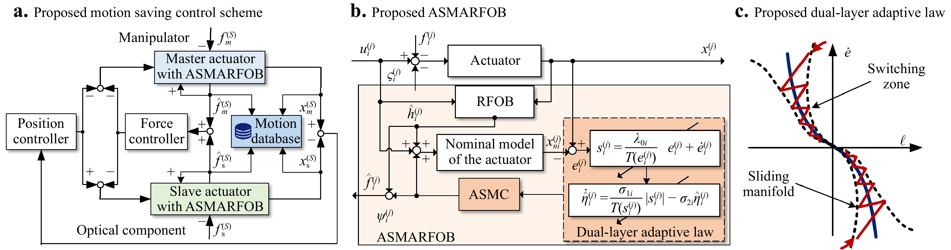
Fig. 2 Proposed motion saving control scheme with ASMARFOB
When MCS contacts the surface of an optical component with a certain stiffness, the manipulation force would change abruptly. The traditional force-sensorless estimator RFOB with low-pass filters can only perform well in low-frequency operations. An ASMARFOB is proposed herein to further improve the bandwidth and accuracy of force estimation in the MCS (Fig. 2b). The ASMARFOB is composed of an RFOB and assistant dual-layer adaptive sliding mode controller (ASMC). The introduction of ASMC can further compensate for the estimation error of the conventional RFOB. The design of dual-layer adaptive strategy in the ASMC seeks to achieve two objectives: the switching gain decreases rapidly as the sliding manifold diminishes, and the sliding manifold converges quickly with the reduction in error; thus, the convergence rate is improved while chattering is reduced (as shown in Fig. 2c).
In the proposed ASMARFOB, the traditional RFOB is applied to estimate the contact force $ \hat{h}_i^{(j)} $ at a relatively low frequency. The estimation is expressed as
$$ \left\{ \begin{array}{l} \hat{h}_i^{(j)}=\zeta_i^{(j)}-l_{i} J_{ni} \dot x_i^{(j)}-l_{i} B_{ni} x_i^{(j)}\\ \dot{\zeta}_i^{(j)}=l_{i}(u_i^{(j)}+l_{i} J_{ni}\dot x_i^{(j)}+l_{i} B_{ni}{x}_i^{(j)})-l_{i}\zeta_i^{(j)}\\ \end{array} \right.$$ (5) where $ \zeta_i^{(j)}, \hat h_i^{(j)} $ and $ l_{i} $ are the state variable, output, and gain of the RFOB, respectively. The estimation error of the RFOB is $ \tilde{h}_i^{(j)}=f_i^{(j)}-\hat{h}_i^{(j)} $.
Assumption 3: Considering the verification capability of the RFOB in compensating for system disturbances and model uncertainties28, there exists an upper bound of $ \tilde{h}_i^{(j)} $ in Eq. 5, thereby satisfying $ |\tilde{h}_i^{(j)}|<\bar{h}_{i}^{(j)} $.
We define an auxiliary subsystem with a nominal control plant as
$$ \begin{array}{*{20}{l}} J_{ni}\ddot{x}_{ni}^{(j)}+B_{ni}\dot{x}_{ni}^{(j)}=u_{i}^{(j)}-\hat{h}_i^{(j)}-\psi_i^{(j)} \end{array} $$ (6) where $ x_{ni}^{(j)} $ is the nominal state of the actuator, and $ \psi_i^{(j)} $ is the output of the ASMC from the slave and master sides.
The ASMC is designed to compensate for the estimation error of the RFOB and obtain force information over a wider bandwidth. The nominal error is defined as $ e_i^{(j)}=x_{ni}^{(j)}-x_i^{(j)} $, and the control objective of the ASMC is $ e_i^{(j)} \to 0 $. Consequently, the observing error of the ASMARFOB is $ f_i^{(j)}-(\hat{h}_i^{(j)}+\psi_i^{(j)})\to 0 $.
$ \psi_i^{(j)} $ is herein defined as
$$ \begin{array}{*{20}{l}} \psi_{i}^{(j)}= -B_{ni}\dot e_i^{(j)} +J_{ni}{\lambda_i \dot e_i^{(j)}}+\hat \eta_i^{(j)} sgn(s_i^{(j)})+\beta_i s_i^{(j)} \end{array} $$ (7) where $ sgn(\cdot) $ is the sign function, and $ \beta_i>0 $. $ \hat \eta_i^{(j)} $ is the adaptive-switching gain, which is an estimate of the upper bound of $ \tilde{h}_i^{(j)} $. Further, $ \lambda_{i}={\lambda_{0i}}/{T(e_i^{(j)})} $, and $ \lambda_{0i}>0 $.
Both the adaptive sliding manifold and switching gain were designed.
The adaptive sliding manifold of ASMC is defined as
$$ \begin{array}{*{20}{l}} s_i^{(j)}=\lambda_{i} e_i^{(j)}+\dot e_i^{(j)} \end{array} $$ (8) The adaptive law of the switching gain is given by
$$ \begin{array}{*{20}{l}} \dot{\hat{\eta}}_i^{(j)}=\dfrac{\sigma_{1i}}{T(s_i^{(j)})}|s_i^{(j)}|-{\sigma_{2i}}\hat{\eta}_i^{(j)},\; (\sigma_{1i},\sigma_{2i}>0) \end{array} $$ (9) A nonlinear function $ T(\cdot) $ is introduced in the design of the sliding manifold and adaptive law, as follows:
$$ \begin{array}{*{20}{l}} T(\cdot) = \text{tanh}(\dfrac{g_T}{|\cdot|}) \end{array} $$ (10) where $ \text{tanh}(\cdot)={\text{sinh}\; (\cdot)}/{\text{cosh}\; (\cdot)}=({e^{(\cdot)} - e^{-(\cdot)}})/({e^{(\cdot)} + e^{-(\cdot)}} )$, and $ g_T\in (0,1) $ is a constant for different sliding manifold and nominal errors from master and slave sides, respectively. Further, $ T(\cdot)\in (0,1) $.
Thus, we obtain:
$$ \begin{array}{*{20}{l}} \hat f_i^{(j)}=\hat h_i^{(j)}+\psi_i^{(j)} \end{array} $$ (11) The control objective of the MSSS is the position synchronisation and balance of the action and reaction forces.
-
In the MRSS, the stored motion data of the master side serve as a virtual master to control the slave side by recapturing its motion. Ideally, the motion information stored in the MCS should be accurately and completely reproduced under these conditions. However, the initial location of the manipulated object can be changed in the MSSS owing to the uncertainty of the operating environment. Consequently, the manipulated information can no longer be matched to the stored information, and the motion-reproducing task fails. SSPSC is employed in the MRSS to solve this issue. The completed manipulation of the MSSS is decomposed into several phases depending on the objectives and is symbolised. Different symbol sequences are combined to adapt to the location uncertainties of the optical component, and a certain phase is reused multiple times for a particular task.
In general, the slave of the MCS is required to track a continuously bounded desired motion command during free motion and to track a desired force command during contact, as expressed by Eq. 12.
$$ u_{s_\sigma}^{(R)} = \left\{ \begin{array}{*{20}{l}} k_{v_1}\bigtriangleup\dot{x}+k_{p_1}\bigtriangleup{x}+k_{f_1}\bigtriangleup{f}, &\sigma=1\\ k_{v_2}\bigtriangleup\dot{x}+k_{p_2}\bigtriangleup{x},& \sigma=2\\ k_{f_3}\bigtriangleup{f}-b_f\dot{x}_s^{(R)},& \sigma=3\\ \end{array} \right. $$ (12) where $ \bigtriangleup{x}=x_m^{(S)}-x_s^{(R)} $, and $ \bigtriangleup{f}=f_m^{(S)}-f_s^{(R)} $. Further, $ k_{p_1} $ and $ k_{p_2} $ are the proportional gains of the position controllers, respectively, whereas $ k_{v_1} $ and $ k_{v_2} $ denote the corresponding gains of the velocity controllers. $ k_{f_1} $ and $ k_{f_3} $ refer to the proportional gain, and $ b_f $ denotes the damping gain of the force controller. Here, $ \sigma $ is a piecewise constant function, called the switching signal. The switch of phases relies on real-time judgement of whether the slave side contacts the object during manipulation. The control strategy for the MRSS is illustrated in Fig. 3a.
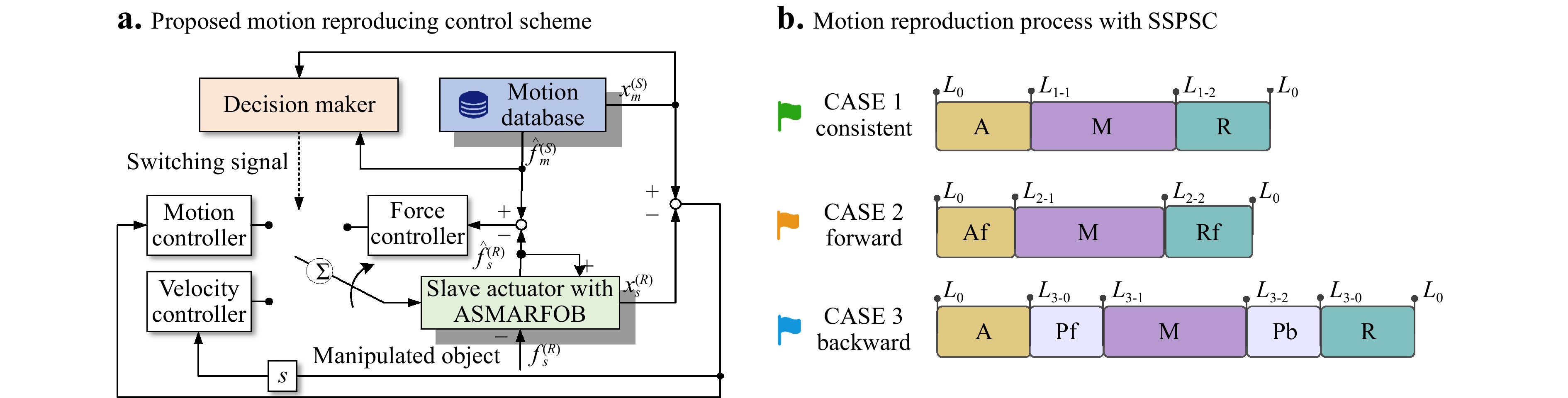
Fig. 3 Proposed motion reproducing control scheme and motion reproduction process with SSPSC
Considering the three typical cases of ‘remain consistent’, ‘move forward’, and ‘move backward’ as examples, the control phases of the manipulation can be composed and symbolised as shown in Fig. 3b.
If the location of the optical component remains unchanged, the data from MSSS are disassembled into three phases according to the different control objectives. During the approach phase, the operator controls the MCS approaching from its initial location $ L_0 $ to physical contact with the manipulated object at $ L_{1-1} $. During the manipulation phase, the end of the slave actuator completes the scheduled manipulations. The return phase refers to the one wherein the operator from the master side controls the end of the slave actuator return to initial location $ L_0 $. These stages are denoted as $ A, M $, and $ R $, respectively. During phases $ A $ and $ R $, a motion-force hybrid controller was applied to the slave side to precisely track the motion trajectory. In phase $ M $, a force controller was applied to ensure the consistency of the manipulated force with the operator. The symbol sequence of motion is $ Af $$ \to $$ M $$ \to Rf $, and the direction of the arrow represents the chronological order. Controller switching occurs when phase changes.
If the initial contact location moved forward to $ L_{2-1}(L_{2-1} \;\; < L_{1-1},L_{2-1} $ is unknown$) $, the end of the slave side would reach and depart the manipulated location ahead of schedule. Approach$ \_ $forward and Return$ \_ $forward phases are supplemented, symbolised as $ Af $ and $ Rf $, respectively, which are actually parts of the phases $ A $ and $ R $ of the free motion. In this case, the symbol sequence of the motion is $ Af $$ \to $$ M $$ \to $$ Rf $.
If the initial contact location moves backwards to $ L_{3-1}(L_{3-1} \;\; > L_{1-1},L_{3-1} $ is unknown$) $, the range of free motion of the slave actuator increases. The Plan$ \_ $forward and Plan$ \_ $backward phases were designed to plan the motion trajectory using a velocity controller between phases $ A,M $ and $ M,R $, symbolised as $ Pf $ and $ Pb $. In this case, the symbol sequence of the motion is $ A $$ \to $$ Pf $$ \to $$ M $$ \to $$ Pb $$ \to $$ R $.
The specific refined control objectives and corresponding control strategies for the different phases are listed in Table 1. The actual location of the object was estimated in real-time and determined using the proposed ASMARFOB with a certain threshold. If the manipulation needs to be repeated multiple times, it can be automatically incorporated into the symbol sequence directly, as shown in Fig. 3b, regardless of whether the location of manipulation object changes each time.
Symbol Phase Control objective Control strategy A Approach Approach from the initial location to the manipulated object hybrid controller Af Approach_forward Approach from the initial location to forward manipulated object hybrid controller M Manipulate Manipulate for a certain period of time under predetermined instructions force controller R Return Return to initial location hybrid controller Rf Return_forward Return forward to initial location hybrid controller Pf Plan_forward Planned forward until physical contact with the manipulated object velocity control Pb Plan_backward Planned backward until back to initial location velocity control Table 1. Detailed design of different symbol phase for motion reproduction
-
This section presents a discussion on the stability of the proposed force estimator ASMARFOB and the synchronisation convergence of the MCS. The switching stability of the MCS among the three controllers for free-motion tracking and constrained motion, which is essential for complete motion reproduction, is then discussed.
-
Theorem 1: Suppose Assumption 1–3 are valid; then, the ultimate boundedness of the proposed ASMARFOB as (11) is achieved. The internal variables of ASMARFOB, $ s_i^{(j)} $ and $ e_i^{(j)} $, are ultimately uniformly bounded and converge to the neighbourhood of zero.
Proof: The proof comprises two steps. We first prove that the sliding manifold (8) reaches the boundary layer containing $ s_i^{(j)}=0 $.
Consider the following Lyapunov function:
$$ \begin{array}{*{20}{l}} V_{s_i}^{(j)} = \dfrac{J_{ni}}{2}(s_i^{(j)})^2+\dfrac{1}{2\sigma_{1i}}(\tilde{\eta}_i^{(j)})^2 \end{array} $$ (13) where $ \tilde{\eta}_{i}^{(j)} = \bar{\eta}_{i}^{(j)}-\hat{\eta}_{i}^{(j)} $ denotes the parameter estimation error. $ \bar{\eta}_{i}^{(j)} $ are the unknown upper bounds of $ \hat{\eta}_{i}^{(j)} $.
Let $ \epsilon_i^{(j)} =\tilde{h}_i^{(j)}+\varsigma_{i}^{(j)} $. According to Assumptions 1 and 2, $ |\epsilon_i^{(j)}|<\bar{\epsilon}_i^{(j)} $, and $ \bar{\epsilon}_i^{(j)}=\bar{h}_{i}^{(j)}+\bar{\varsigma}_{i}^{(j)} $.
Subsequently, the derivative of $ V_{s_i}^{(j)} $ becomes
$$ \begin{aligned} \dot{V}_{s_i}^{(j)}=&J_{ni}s_i^{(j)}\dot{s_i}^{(j)}+\frac{1}{\sigma_{1i}}\tilde{\eta}_i^{(j)}\dot{\tilde{\eta}}_i^{(j)}\\ =&s_i^{(j)}[\epsilon_i^{(j)}-\psi_i^{(j)}+(J_{ni}{\lambda_i}-B_{ni})\dot e_i^{(j)}]-\frac{1}{\sigma_{1i}}\tilde{\eta}_i^{(j)}\dot{\hat{\eta}}_{i}^{(j)}\\ =&s_i^{(j)}\epsilon_i^{(j)}-\hat{\eta}_{i}^{(j)}|s_i^{(j)}|-\beta_i (s_i^{(j)})^2-\frac{1}{\sigma_{1i}}\tilde{\eta}_i^{(j)}\dot{\hat{\eta}}_{i}^{(j)}\\ \leq&(\bar{\epsilon}_i^{(j)}-\hat{\eta}_{i}^{(j)}-\beta_i|s_i^{(j)}|-\frac{\tilde{\eta}_i^{(j)}}{T(s_i^{(j)})})|s_i^{(j)}|+\frac{\sigma_{2i}}{\sigma_{1i}}\tilde{\eta}_i^{(j)}\hat{\eta}_i^{(j)}\\ \end{aligned} $$ (14) Because $ \tilde{\eta}_{i}^{(j)}\hat{\eta}_{i}^{(j)}=(\bar{\eta}_{i}^{(j)}-\hat{\eta}_{i})^{(j)}\hat{\eta}_{i}^{(j)} $, its maximum is $ (\bar{\eta}_{i}^{(j)})^2/4 $ when $ \hat{\eta}_{i}^{(j)} = \bar{\eta}_{i}^{(j)}/2 $, and $ \hat{\eta}_{i}^{(j)}+{\tilde{\eta}_i^{(j)}}/{T(s_i^{(j)})}\ge\bar{\eta}_i^{(j)} $.
Set $ \eta_{si}^{(j)}=({\sigma_{2i}}/{\sigma_{1i}})({(\bar{\eta}_{i}^{(j)})^2}/{4}) $. Then, $ \exists \Psi_{1i}^{(j)} = $ $ inf(\beta_i|\lambda_{0i} e_i^{(j)}+\dot e_i^{(j)}|) $, and $ \Psi_{si}^{(j)}=\Psi_{1i}^{(j)}+\bar{\eta}_i^{(j)}-\bar{\epsilon}_i^{(j)} $. In this study, $ \Psi_{si}^{(j)}\geq 0 $ was be guaranteed by appropriately setting certain parameters.
Hence, it follows that
$$ \begin{array}{*{20}{l}} \begin{aligned} \dot V_{s_i}^{(j)}\leq &-\Psi_{si}^{(j)}|s_i^{(j)}|+\eta_{si}^{(j)} \\ \leq & -(1-\delta_{si}^{(j)})\Psi_{si}^{(j)} |s_i^{(j)}|, \forall |s_i^{(j)}|\geq \frac{\eta_{si}^{(j)}}{\delta_{si}^{(j)} \Psi_{si}^{(j)}} \end{aligned} \end{array} $$ (15) where $ 0<\delta_{si}^{(j)}<1 $. The sliding manifold $ s_i^{(j)} $ reaches the boundary layer as follows:
$$ \begin{array}{*{20}{l}} \Omega_{s_i}^{(j)} = \{|s_i^{(j)}|\leq \dfrac{\eta_{si}^{(j)}}{\delta_{si}^{(j)} \Psi_{si}^{(j)}}\} \end{array} $$ (16) Inside the boundaries of Eq. 16, $ \dot e_i^{(j)}=-({\lambda_{0i}}/{T(e_i^{(j)})}) e_i^{(j)}+ s_i^{(j)} $. Then, the derivative of $ V_{e_i^{(j)}}={1}/{2}(e_i^{(j)})^2 $ satisfies
$$ \begin{array}{*{20}{l}} \begin{aligned} \dot V_{e_i^{(j)}}=& -\frac{\lambda_{0i}}{T(e_i^{(j)})} (e_i^{(j)})^2+e_i^{(j)}s_i^{(j)}\\ \leq& -\lambda_{0i} |e_i^{(j)}|^2+\frac{\eta_{si}^{(j)}}{\delta_{si}^{(j)} \Psi_{si}^{(j)}}|e_i^{(j)}|\\ \leq& -(1-\delta_{e_i^{(j)}})\lambda_{0i}|e_i^{(j)}|^2, \forall |e_i^{(j)}|\geq \frac{1}{\delta_{e_i^{(j)}}\lambda_{0i}}\frac{\eta_{s_i}^{(j)}}{\delta_{s_i}^{(j)} \Psi_{s_i}^{(j)}} \end{aligned} \end{array} $$ (17) where $ 0<\delta_{e_i^{(j)}}<1 $.
Eq. 17 indicates that the estimation error of the ASMARFOB $ e_i^{(j)} $ reaches the set $ \Omega_{e_i^{(j)}} = \{|e_i^{(j)}|\leq ({\eta_{s_i}^{(j)}}/ {\delta_{e_i^{(j)}}\lambda_{0i}\delta_{s_i}^{(j)} \Psi_{s_i}^{(j)}}) \}$, and $ e_i^{(j)} $ is ultimately bounded.
Remark: As indicated by Eqs. 15 and 17, the proposed ASMARFOB in Eq. 11 is uniformly ultimately bounded. Thus, the trajectory of the nominal error $ e_i^{(j)} $ reaches the sliding surface, its internal variables $ s_i^{(j)} $ and $ e_i^{(j)} $ are ultimately uniformly bounded, and $ \bigtriangleup f_{i}^{(j)}=\hat f_{i}^{(j)}-f_{i}^{(j)}\to 0 $.
-
The position-force bilateral control laws in the MSSS are as follows:
$$\left\{ \begin{array}{*{20}{l}} u_{m}^{(S)} =- k_{v_1}\dot{e}_p-k_{p_1}{e_p}+k_{f_1}e_f + \hat f_m^{(S)}\\u_s^{(S)}=k_{v_1}\dot e_p +k_{p_1}e_p+k_{f_1}e_f+\hat f_s^{(S)}\end{array}\right. $$ (18) where $ e_p=x_m^{(S)}-x_s^{(S)} $ is the position synchronisation error between the master and slave sides, and $ e_f=f_m^{(S)}+f_s^{(S)} $ is the resultant residual force.
According to Eq. 3, and Eq. 18,
$$ \begin{array}{*{20}{l}} \begin{aligned} J_{n}\ddot{e}_p+(B_{n}+2k_{v_1})\dot{e}_p+2k_{p_1}e_p=&\bigtriangleup f_{m}^{(S)}-\bigtriangleup f_{s}^{(S)}\\&-\varsigma_{m}^{(S)}+\varsigma_{s}^{(S)} \end{aligned} \end{array} $$ (19) On the basis of the analysis detailed in the previous subsection and Assumption 1
$$ \begin{array}{*{20}{l}} J_{n}\ddot{e}_p+(B_{n}+2k_{v_1})\dot{e}_p+2k_{p_1}e_p\to 0 \end{array} $$ (20) Eq. 20 is $ e_p\to 0 $. Consequently, the objective of position synchronisation is realised.
Furthermore, based on Eqs. 3 and 18, we derive
$$ \begin{array}{*{20}{l}} J_{n}(\ddot{x}_m^{(S)}+\ddot{x}_s^{(S)})+B_{n}(\dot{x}_m^{(S)}+\dot{x}_s^{(S)})\to2k_{f_1}e_f \end{array} $$ (21) When $ e_p\to0 $, assuming $ {x}_m^{(S)}={x}_s^{(S)}={x}^{(S)} $, Eq. 21 can be rewritten as
$$ \begin{array}{*{20}{l}} J_{n}\ddot{x}^{(S)}+B_{n}\dot{x}^{(S)}\to k_{f_1}(f_m^{(S)}+f_s^{(S)}) \end{array} $$ (22) Eq. 21 indicates that the manipulated and environmental forces act on the master and slave actuators, respectively. When the slave side is in contact with the high-stiffness optical component, the positions of the MCS remain constant, $ f_m^{(S)}+f_s^{(S)}\to 0 $, and the objective of force synchronisation is realised.
In the MRSS, the stored master motion data serve as command input. It may be easily deduced that the slave side may track the stored data on the basis of Eq. 12.
-
To examine the switching stability, the closed-loop dynamic model in Eq. 12 is reformulated into a state-space switching model. According to the Kelvin–Voigt contact model, the stored force data $ f_m^{(R)} $ can be equivalently mapped to the motion data $ x_m^{(R)} $ as Eq. 23. In this case, $ x_m^{(R)} $ represents the ‘virtually’ desired trajectory of the force controller corresponding to the desired manipulating force $ f_m^{(R)} $.
$$ \begin{array}{*{20}{l}} \hat{k}_ex_m^{(R)}+\hat{b}_e\dot{x}_m^{(R)}=f_m^{(R)}, f_m^{(R)}>0 \end{array} $$ (23) where $ \hat{k}_e $ and $ \hat{b}_e $ are the estimated values of $ k_e $ and $ b_e $, respectively.
The following assumption can be reasonably established under Assumption 2.
Assumption 4: The desired position data $ x_m^{(R)} $ and its velocity $ \dot{x}_m^{(R)} $ are continuous, and its acceleration $ \ddot{x}_m^{(R)} $ is piecewise-continuous and bounded.
Consequently, Eq. 23 can be rewritten as
$$ \begin{array}{*{20}{l}} k_ex_m^{(R)}+b_e\dot{x}_m^{(R)}+l_f=f_m^{(R)}, f_m^{(R)}>0 \end{array} $$ (24) where $ l_f=(\hat{k}_e-k_e)x_m^{(R)}+(\hat{b}_e-b_e)\dot{x}_m^{(R)} $ denotes the bounded estimation error. Given that the relationships in Eq. 24 is used only for the stability analysis, the accuracy of $ \hat{k}_e, \hat{b}_e $ does not affect the stability of the control system, as indicated by Eq. 12.
The tracking error matrix of the MRSS is defined as
$$ \begin{array}{*{20}{l}} e= \begin{bmatrix} e_1\\ e_2 \end{bmatrix} =\begin{bmatrix} x_m^{(R)}-{x}_s^{(R)}\\ \dot{x}_m^{(R)}-\dot{x}_s^{(R)} \end{bmatrix} \end{array} $$ (25) Subsequently, the closed-loop dynamic models in Eq. 12 for the slave side in the MCS can be rewritten as the switched state-space model
$$ \begin{array}{*{20}{l}} \dot{e}=A_\sigma e+Nr_\sigma= \begin{bmatrix} 0 &1\\ -k_\sigma &-h_\sigma\end{bmatrix}e+Nr_\sigma,\sigma\in\{1,2,3\} \end{array} $$ (26) where $ N=[0, 1]^T $. Further,
$$ \begin{array}{*{20}{l}} k_1=\dfrac{(1+k_{f_1})k_e+k_{p_1}}{J_{ns}},\;h_1=\dfrac{(1+k_{f_1})b_e+k_{v_1}+B_{ns}}{J_{ns}} \end{array} $$ (27) $$ \begin{array}{*{20}{l}} r_1=\ddot{x}_m^{(R)}+\dfrac{B_{ns}+b_e}{J_{ns}}\dot{x}_m^{(R)}+\dfrac{k_e}{J_{ns}}x_m^{(R)}-\dfrac{k_{f_1}}{J_{ns}}l_f+\dfrac{1}{J_{ns}}\varsigma_s^{(R)} \end{array} $$ (28) $$ \begin{array}{*{20}{l}} k_2=\dfrac{k_{p_2}}{J_{ns}},\;h_2=\dfrac{k_{v_2}+B_{ns}}{J_{ns}},\;r_2=\ddot{x}_m^{(R)}+\dfrac{B_{ns}}{J_{ns}}\dot{x}_m^{(R)}+\dfrac{1}{J_{ns}}\varsigma_s^{(R)} \end{array} $$ (29) $$ \begin{array}{*{20}{l}} k_3=\dfrac{(1+k_{f_3})k_e}{J_{ns}},\; h_3=\dfrac{(1+k_{f_3})b_e+b_f+B_{ns}}{J_{ns}} \end{array} $$ (30) $$ \begin{array}{*{20}{l}} r_3=\ddot{x}_m^{(R)}+\dfrac{b_f+B_{ns}+b_e}{J_{ns}}\dot{x}_m^{(R)}+\dfrac{k_e}{J_{ns}}x_m^{(R)}-\dfrac{k_{f_3}}{J_{ns}}l_f+\dfrac{1}{J_{ns}}\varsigma_s^{(R)} \end{array} $$ (31) The value of $ r_\sigma $ can be considered the system input in Eq. 26 and bounded by Assumption 4.
It can be deduced that $ k_\sigma > 0 $, and $ h_\sigma>0 $. Therefore, $ A_\sigma\; (\sigma\in\{1,2,3\}) $ is the Hurwitz problem: When $ r_i\equiv0 $, the system represented by Eq. 26 can be rewritten as
$$ \begin{array}{*{20}{l}} \dot{e}=A_\sigma e= \begin{bmatrix} 0 &1\\ -k_\sigma &-h_\sigma\end{bmatrix}e,\sigma\in\{1,2,3\}, \end{array} $$ (32) where $ e\in \mathbb{R}^2 $ is the state vector of the switching system.
In the proposed design, $ \sigma\in\{1,2,3\} $. There are three possible switching scenarios. Considering that switching between $ \sigma_2 $ and $ \sigma_3 $ is a switch between free and constrained motion, its switching stability is discussed as follows. The switching stability of other switches can be directly deduced by following the same steps.
Consider the switched system $ \dot{e}=A_\sigma e, \;\forall e\in \Psi_\sigma, \sigma\in\{2,3\} $. We define a positive-definite Lyapunov function $ V_\sigma=e^Te>0 $ and its time derivative $ \dot{V}_\sigma=e^T(A_\sigma^T+A_\sigma)e= -2h_\sigma e_2^2+ 2(1-k_\sigma)e_1e_2 $. Assume that $ k_3>k_2 $. It follows that $ \dot{V}_2>\dot{V}_3 $ if $ e_2((k_2-k_3)e_1+(h_2-h_3)e_2)< 0 $, and vice versa. Let $ \Psi_2=\{e\in\mathbb{R}|e_2((k_2-k_3)e_1+(h_2-h_3)e_2)\le 0\} $ and $ \Psi_3= \{e\in\mathbb{R}|e_2((k_2-k_3)e_1+(h2-k3)e_2)> 0\} $. Two switching surfaces $ e_2=0 $ and $ (k_2-k_3)e_1+(h_2-h_3)e_2=0 $ are obtained to characterise the switching.
According to the analysis in Ref. 29, $ k_\sigma,h_\sigma>0 $ for $ \sigma\in\{2,3\} $. Let $ \bigtriangleup k:= k_2-k_3<0 $ and $ \bigtriangleup h:= h_2-h_3 $. The origin of the unperturbed linear system in Eq. 32 is the global uniform exponential stability (GUES) if $ k_\sigma $ and $ h_\sigma $ satisfy certain constraint relationships associated with its eigenvalue.
Moreover, consider the perturbed system in Eq. 26 with piecewise-continuous bounded input $ r_\sigma $. If the origin of the unperturbed system in Eq. 32 is GUES for arbitrary $ x_m^{(R)} $ satisfying Assumption 4, $ x_m^{(R)} $ encodes the information of $ f_m^{(R)} $ during the contact; thus, $ x_s^{(R)}\to x_m^{(R)} $ and $ f_s^{(R)}\to f_m^{(R)} $ exponentially. Then, the system in Eq. 26 is input-to-state stable (ISS). The response in Eq. 26 deviates from the response in Eq. 32; however, the response of the system in Eq. 26 is bounded, depending on the norm $ Nr_\sigma $.
-
To illustrate the effectiveness of the proposal, the motion copy and reproduction performance was simulated.
Motion saving During the MSSS, a virtual manipulated force is generated on the master side. Through bilateral control, the slave side from its initial position contacts a virtual stiff optical component with $ k_e=5000 $ and $ b_e=15 $ at the position of 0.25 mm and then returns to the initial position. The motion trajectories of the MCS with RFOB and the proposed ASMAFROB are shown in Fig. 4a. The shadowed areas with different colours represent the corresponding phases of motion.
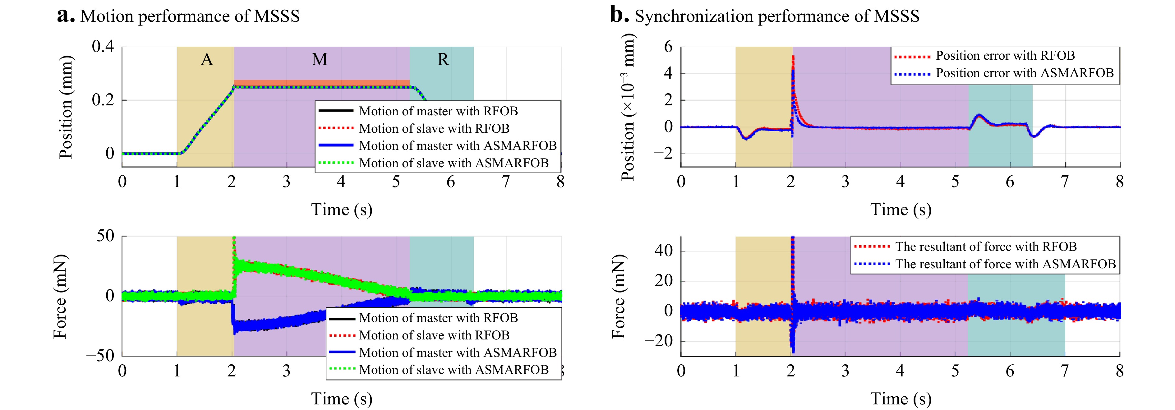
Fig. 4 Simulated trajectory of the MSSS
The position and force synchronisation errors of the MCS with the traditional RFOB and the proposed ASMARFOB are shown in Fig. 4b, respectively. A comparison of the motion performance during motion space switching, transitioning from free to constrained, is presented in Table 2. The results demonstrate that the proposed method using ASMARFOB exhibits superior force estimation and synchronisation characteristics. This enables a more rapid response to varying environmental stiffness with a smaller estimated error, thereby facilitating faster attainment of stable motion control performance in terms of the root-mean-square error (RMSE), settling time, overshooting of position synchronisation, and RMSE of force synchronisation.
Method Position RMSE Settling time Maximum Overshoot Force RMSE RFOB 0.16 μm 0.281 s 5.3 μm 14.87 mN Proposal 0.11 μm 0.163 s 4.4 μm 13.93 mN Table 2. Motion performance comparison during motion space switching
Motion reproducing In the MRSS, the stored motion data are used as a virtual master, and the slave actuator is simulated to reproduce completed manipulating trajectories. Considering that unknown changes in the location of the optical component affect the exact motion reproduction, the following three cases were considered, and the control scheme proposed in20 was employed for comparison.
Case 1: Initial contact position remains consistent
If the initial contact position of the manipulated object remains at 0.25 mm, the simulated trajectory of reproduced motion and the resultant of force are as shown in Fig. 5. Both methods exhibited good motion replication performance.
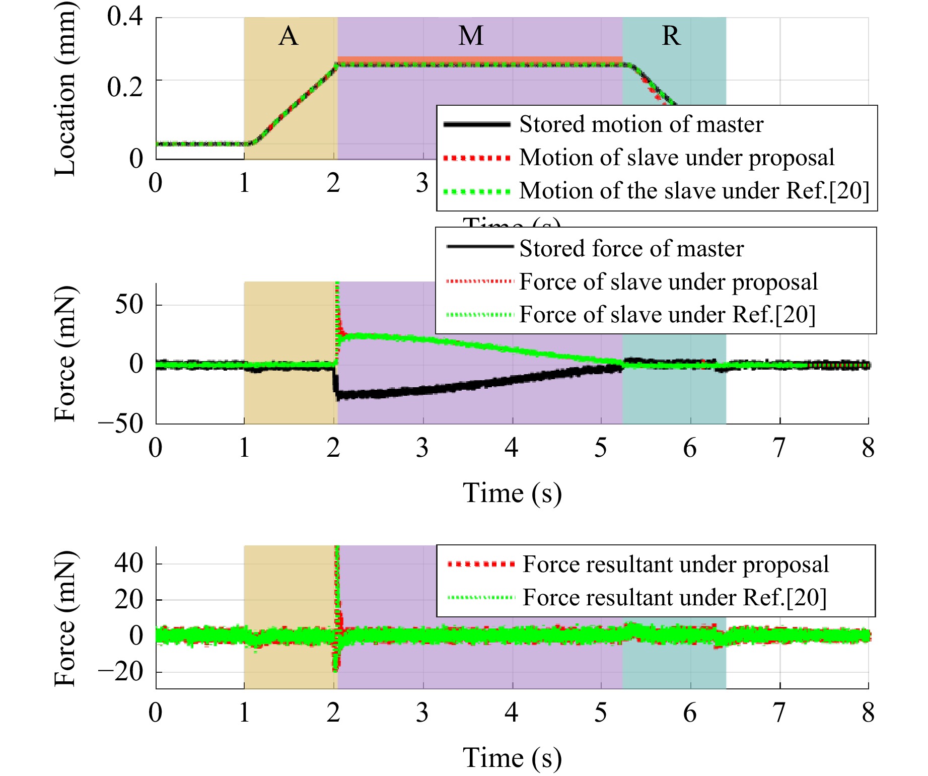
Fig. 5 Simulated trajectory of MRSS under case 1
Case 2: Initial contact position moved forward
When the slave actuator contacted the manipulated object in advance at 0.2 mm, its controller immediately switched from the hybrid controller to force controller and reproduced the stored manipulation. The simulated trajectory of the reproduced motion and the resultant force of the MCS are presented in Fig. 6.
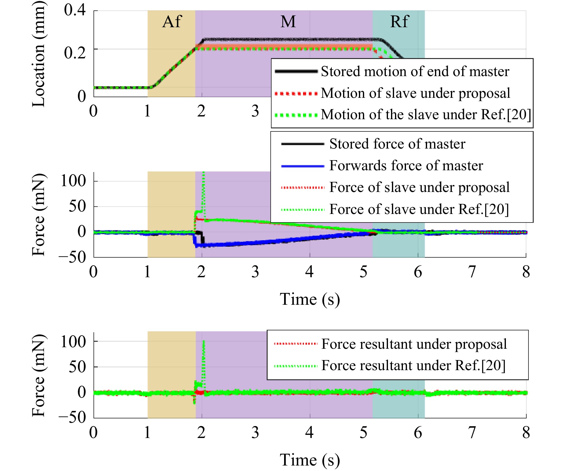
Fig. 6 Simulated trajectory of the MRSS under case 2
Evidently, reproduction failure happens with a large overshoot at the beginning the manipulation under20, whereas the resultant of force during phase M under the proposed method is nearly zero, achieving good transparency and motion reproduction performance.
Case 3: Initial contact position moved backward
If the manipulated object was moved backwards to 0.3 mm, no contact force would be detected when the slave actuator reached the stored contact position. Then, the velocity controller would be applied at a constant velocity until the slave side contacted the optical component, and the controller switched to the force controller. The simulated motion trajectory is shown in Fig. 7.
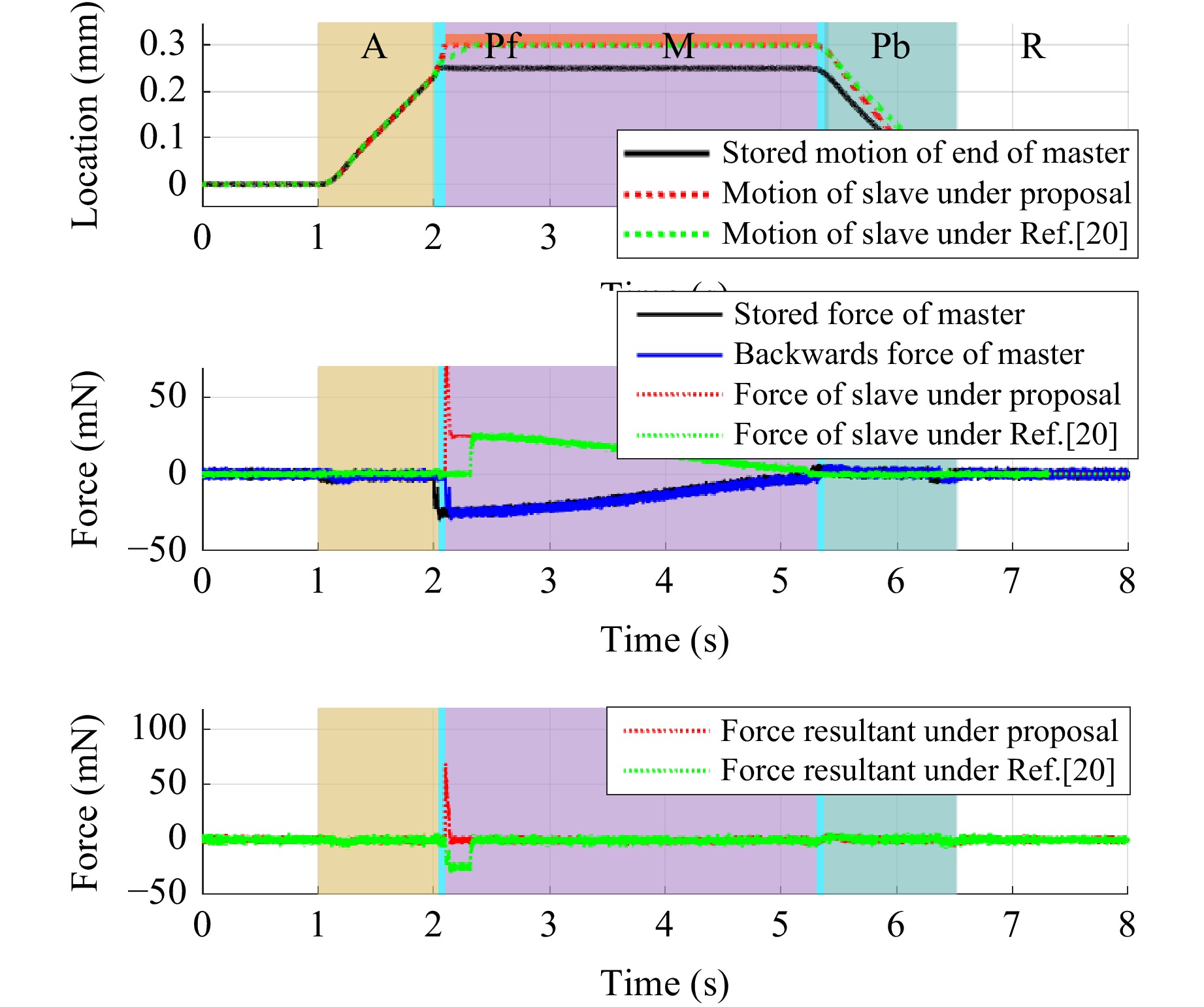
Fig. 7 Simulated trajectory of MRSS under case 3
The comparative performance of motion replication during the manipulation phase is presented in Table 3. The manipulation consistency is defined as the percentage of time for which the resultant force is within the range of ±5 mN over the entire manipulation phase. It was found that the method in Ref. 20 exhibits greater manipulation inconsistency in the three different cases. In contrast, the proposed method demonstrated a smaller RMSE and maximum error, ensuring over 98% motion consistency.
Table 3. Performance indices of motion replication during the manipulation phase
-
The proposed approach was further verified experimentally on a principal prototype for optical polishing. The control algorithms were programmed in the C language on an embedded microcontroller with the sampling time of 1 ms. The hardware system exhibited good real-time performance and portability. The position responses of the prototype were measured using encoders, and the manipulation angle corresponding to the operating torque was obtained. During the MSSS, the position and force data are stored in the motion data memory at each sampling time. These data are used as the virtual master system of the motion reproduction system. The experimental setup is shown in Fig. 8.
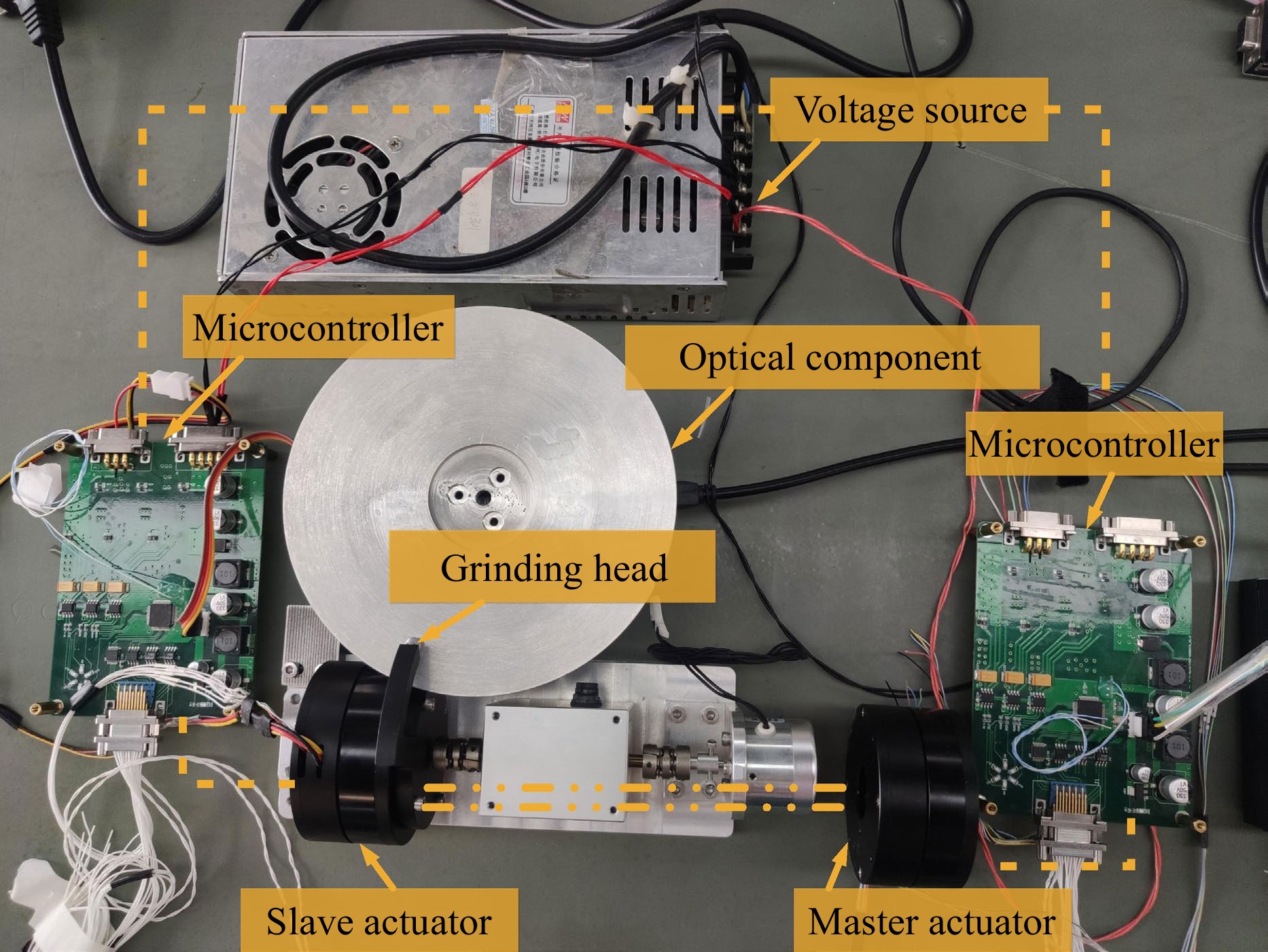
Fig. 8 Experimental setup of the MCS prototype
Motion saving During the MSSS, a technician operates the end of the master actuator by using force-position bilateral control of the MCS, and the end of the slave actuator moves from its initial position to contact with the optical component, completing a period of the manufacturing process with fine force control and then returning to the initial position. The motion trajectory of the MCS is shown in Fig. 9. The location of the manipulated object was set to 0.4008° in this experiment, and the RMSE of the resultant force was 0.01 Nm. After the entire operation was completed, the motion data of both sides were saved in the system memory.
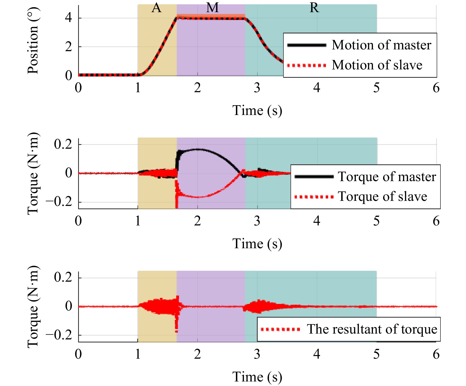
Fig. 9 Motion trajectory of MSSS
Motion reproducing In the MRSS, the stored motion data is used as a virtual master, and the slave actuator is controlled to reproduce completed manipulating trajectories. Considering that unknown changes in the initial position of the optical component affect the exact motion reproduction, the following three cases are considered.
Case 1: Initial contact location remains consistent
If the initial contact position of the manipulated object remains the same as that during the motion-saving stage, the motion trajectory of the slave actuator is shown in Fig. 10.
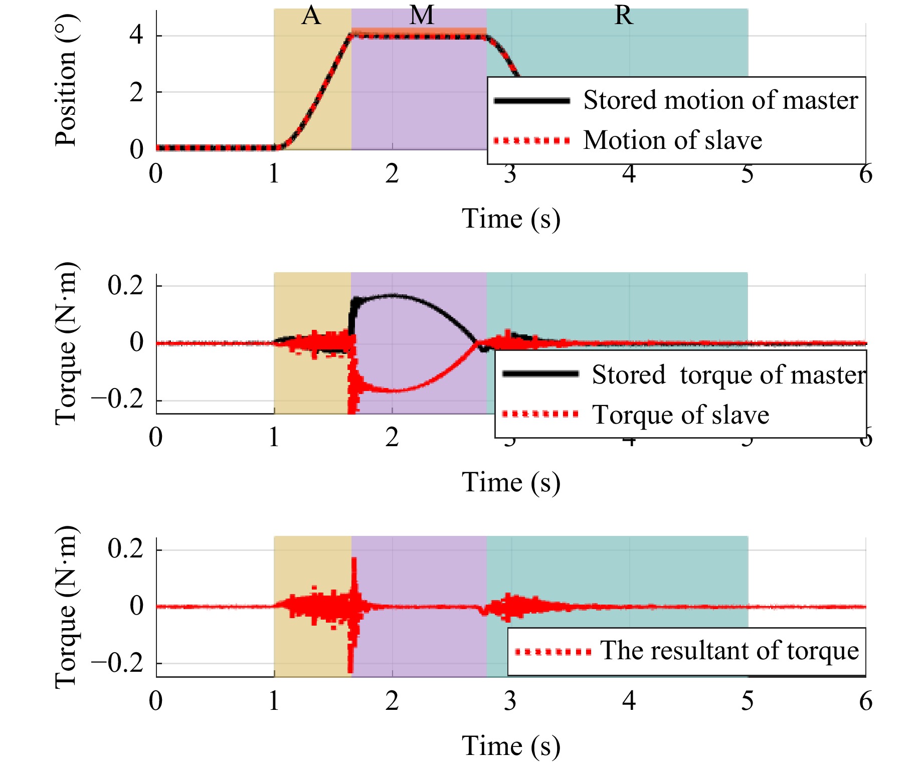
Fig. 10 Trajectory of MRSS under case 1
After analysis, the RMSE of the resultant of force under the proposed method is 0.0163 Nm, achieving good transparency and motion reproduction performance.
Case 2: Initial contact location moved forward
When the end of the slave actuator contacts the manipulated object in advance, the controller of the slave actuator immediately switches from the position controller to the force controller and reproduces the manipulation based on the stored master data. The trajectory of the motion in this case is shown in Fig. 11.
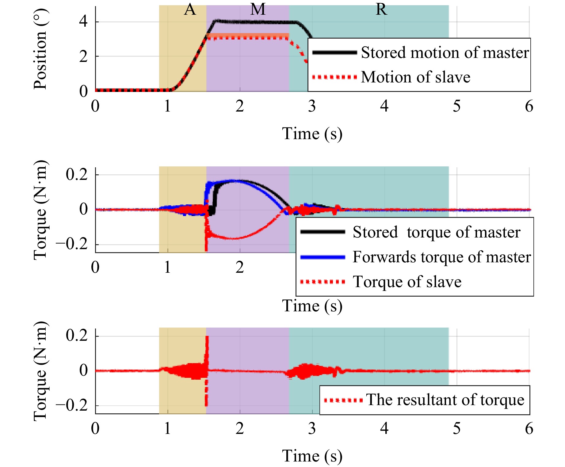
Fig. 11 Trajectory of MRSS under case 2
Analysis shows that the manipulation location moves forward by 0.92° in this experiment, the RMSE of the resultant of force is 0.0182 Nm. The stored manipulation can be reproduced well using the proposed method when the manipulation location is moved in advance.
Case 3: Initial contact location moved backward
If no contact force was detected when the slave actuator reached the stored contact position, it implies that the actual location of the optical component is moved backward. Phases $ Pf $ and $ Pb $ were additionally designed. The trajectory of motion in this case is shown in Fig. 12.
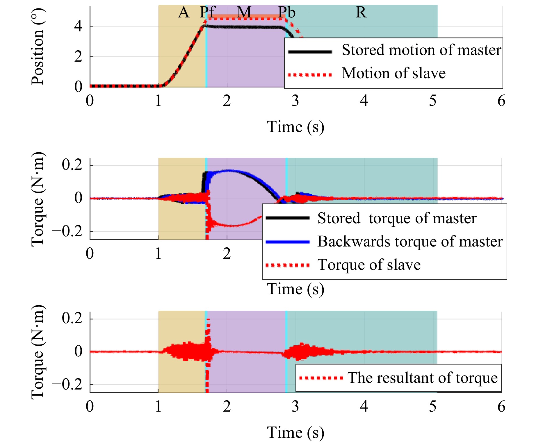
Fig. 12 Trajectory of MRSS under case 3
Data analysis reveals that the manipulation location moves backward by $ 0.0558^\circ $ in this case, the RMSE of the resultant of force under the proposed method is $ 0.0226\; \rm{Nm} $, and the stored manipulation is reproduced well with high manipulation consistency under the proposed method.
-
The simulation and experimental results indicate that the proposed method can achieve high-precision motion copy and high consistent motion reproduction with location uncertainties. During the manipulation phase, the MCS with the proposed SSPSC and ASMARFOB achieved good transparency and motion reproduction performance.
Fig. 4 and Fig. 9 show that good position and force synchronisation are achieved between the master and slave side in the MCS. Compared to the traditional RFOB, the control error of the proposed ASMARFOB with the dual-layer adaptive law is markedly decreased, particularly when the motion space is switched. The results indicate that reductions of more than 42% in settling time, 17% in overshoot, and 26% in force RMSE were achieved by the proposed method as compared with the traditional RFOB. Faster attainment of stable motion control performance was facilitated.
It can be observed in Figs. 5-7, Figs. 10-12, regardless of how the contact location changes, under the proposed SSPSC, favourable force reproduction performance can be achieved. Stored and reproductive forces satisfy the laws of action and reaction. This is because the proposed scheme provides a more rational understanding and reproduction of multidimensional motion and tactile information of the technician's manipulation characteristics. The decomposed symbol-sequence-based phases make intelligent optical manufacturing processes more flexible and adaptable. The minor differences between the simulated and experimental data may be attributed to uncompensated disturbances, model uncertainties, and sensor noise from the actual prototype.
As shown in Table 3, the manipulation consistency is improved by the proposed method, and it exhibits satisfactory robustness against location uncertainties and switching of the motion space. Compared with the method in Ref. 20, over 98% motion consistency was ensured, and a smaller RMSE and maximum error were guaranteed. In the manufacturing scenario considered in this study, better performance in skill learning and motion reproduction was achieved using the proposed scheme. The greater the contact location deviation, the more evident was the advantage of the proposed method.
-
To address problems of the location uncertainties and motion spaces switching confronting the application of motion copy method to intelligent optical manufacturing, a symbol sequence-based phase switch control scheme was devised in this study. Entire technician’s manipulation process was decomposed, symbolised, rearranged, and reproduced according to the detailed manufacturing characteristics. The hybrid, force, and velocity control strategies were separately designed. To avoid space constraints on the force sensor and improve the force-sensing accuracy and bandwidth, a force-sensorless adaptive sliding-mode-assisted reaction force observer was established, wherein a novel dual-layer adaptive law was designed for better performance in fine force sensing and control. Experiments were conducted on a principal prototype, and the reproduction error was reduced as compared to other methods. The results of this study provide theoretical and practical support for research on motion copying and reproduction with location uncertainties and are promising for the process improvement of intelligent optical manufacturing.
The actual grinding and polishing processes for complex optical components may be implemented by experienced technicians with multi-degree-of-freedom manipulations. In this scenario, the proposed method may face challenges caused by coupling and cooperation between different degrees of freedom. To address these challenges, in the future, we will collect and analyse the multidimensional motion characteristics of experienced technicians and investigate a more accurate and intelligent motion-copying method for multi-degree-of-freedom MCS systems. In addition, we will further consider the impact of adhesives and their uncertainties on motion learning and reproduction in intelligent optical manufacturing.
-
This work was supported in part by the National Science Foundation of China, under grant numbers T2122001 and 12203049, in part by the Key Research Program of Frontier Sciences, CAS, under grant number ZDBS-LY-JSC044, and in part by the Youth Innovation Promotion Association of the Chinese Academy of Sciences under Grant number 2023230.

 DownLoad: