Deep holography

DNN can be regarded as a category of machine learning algorithms that are designed to extract information from raw data and represent it in some sort of model⁴². Specifically, a neural network (NN) is built on a collection of connected units called artificial neurons, which are typically organized in layers, an idea somehow inspired by the biological neuron in the mammalian brain. As schematically shown in Fig. 1a, a modern NN consists of three kinds of layers: the input layer, the output layer, and the hidden layers. The input layer usually represents the signal to be processed and the output layer represents the expected result that one wishes the network to produce. So the widths ($ P $), i.e., the number of neurons, of these two layers are task-specific. Data processing is mainly performed by the hidden layers that lay between the input and the output layers. Each successive hidden layer uses the outputs from its upstream layers as its input, processes it, and then passes the result to a downstream layer. In this manuscript, we use the digit $ l = 1,\ldots,L $ to enumerate the layers, where $ L $ is called the depth of the NN. A neural network is deep if it has many layers. The depth of modern deep neural networks ranges from 8 layers in AlexNet¹⁰⁰ to 152 layers in ResNet¹⁰¹, which has the potential to increase to more than 1000 layers¹⁰². The requirement of computation resource dramatically increases along with the up-scaling of the DNN, i.e., the number of hidden layers and hidden neurons. For example, a neural network used for DH have a depth up to 20 layers in a typical proof-of-principle demonstration⁵². It usually takes tens of hours to train on a training set consisting of about thousands of holograms with a modern graphic workstation. Unfortunately, given a problem to be solved by DNN, it is not trivial at all to determine how deep it should be^103,104. Hornik has proved that, for any continuous function $ {\boldsymbol{y}} = f({\boldsymbol{x}}) $, where $ {\boldsymbol{x}} $ and $ {\boldsymbol{y}} $ are data (vectors) in the Euclidean or non-Euclidean space, there is always an NN, no matter how shallow it is, that can approximate the function $ f $ with an infinitesimal error, i.e., $ {\rm{NN}}\{{\boldsymbol{x}}\} \rightarrow {\boldsymbol{y}} $, provided that it is sufficiently wide¹⁰⁵. Practically, however, one still needs a good rule of thumb to configure the number of layers ($ L $) and the numbers of neurons in each layer $ \left(P^{(l)}\right) $. It is commonly believed that the performance of DNN is heavily dependent on the network architecture, which is defined in part by $ L $, $ P^{(l)} $, and the types of connections between layers, the quality of the raw data, and the technique to train the network on them.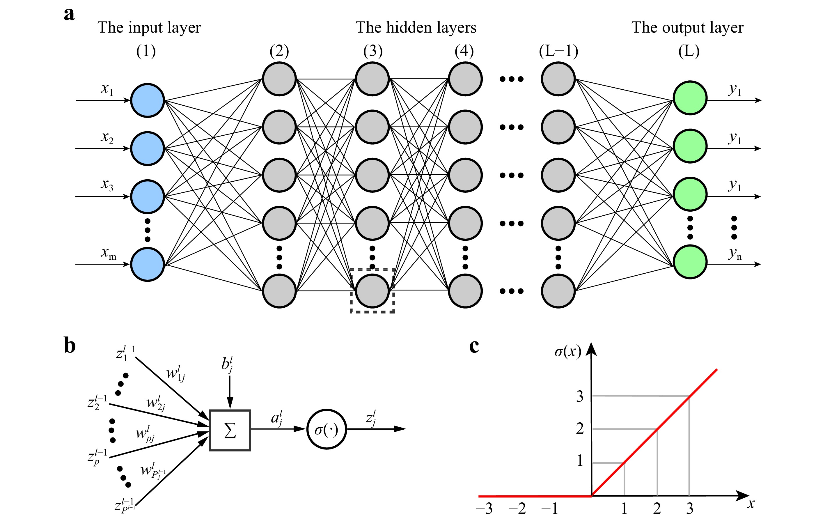

Fig. 1  A conceptual architecture of DNN.

Perhaps the most well-known and easiest to understand DNN is the so-called feedforward neural networks. The architectures of all the other DNNs that are widely used in holography^{51−56,58−62,64−81} are developed on the base of it. Thus it is worthy of discussing it in detail.

As shown in Fig. 1a, a feedforward neural network, or multilayer perceptron (MLP) has one input layer, one output layer, and one or many hidden layers. Each layer may have a different number of neurons called the perceptron. The connections between the neurons in the layers form an acyclic graph¹⁰⁶. The objective of a feedforward neural network is to optimize an NN model $ f_{\rm{NN}} $ that approximates a continuous function $ f $, which maps $ {\boldsymbol{x}} $ in the input space to $ {\boldsymbol{y}} $ in the output space through a set of parameters $ \Theta $ that are learned from the raw data.

The basic unit in a DNN is the artificial neuron. As shown in Fig. 1b, an artificial neuron simply calculates the weighted sum of all the quantities outputted from the neurons in its immediately upstream layer, and passes the resulting quantities to the neurons in the next layer. Let us take the $ j^{\rm{th}} $ neuron at the $ l $ layer for example, the input to this neuron can be written as^41,42

where $ z_p^{(l-1)} $ is the output from the $ p^{\mathrm{th}} $ neuron at the $ (l-1)^\mathrm{th} $ layer, $ w_{pj}^{(l)} $ is the weighting factor that connects these two neurons, and $ b_j^{(l)} $ is a bias. The values of the network parameters $ w_{pj}^{(l)} $ and $ b_j^{(l)} $ are to be learned from a set of raw data called the training set. One can think of their values as the connection strengths between the two neurons. The $ j^{\rm{th}} $ neuron at the $ l $ layer then can be activated if the quantity $ a_j^{(l)} $ is significant (for example, $ >0 $), and this value is passed on to the next layer. Otherwise, this neuron is dead, and should have no contribution to the neurons in the downstream layer. Analogously, one can think of the input signal being an electric current that flows through the network from the input layer to the output layer. Each neuron in the hidden layers acts like a gate that controls the amount of incoming current that is allowed to pass through to the downstream neurons. The “gate” function in a NN is not just a simple “0” and “1” binary function as in the digital electric circuit, but has a form of an activation function. Fig. 1c plots the Rectified Linear Unit (ReLU), which is one of the most important activation function nowadays used in DNN. It is defined as⁴²

ReLU is widely employed in most of the modern neural network architectures, as it has a number of benefits over other old-fashioned activation functions such as Sigmoid and Tanh⁴²: (a) It can be applied to minimize the interaction effects; (b) It is simple and easy to compute, and thus leads to an increment of efficiency in the network training; (c) It helps avoid the vanishing gradient problem; and (d) It is sparsely activated because the output is zero for all negative inputs. However, ReLU sometimes dies, referring to the situation that an neuron has a zero activation value. This dying ReLU issue causes slow-learning because the optimization algorithm is gradient-based and does not adjust the unit weights if the gradient is zero in an inactive neuron. Thus, extensions and alternatives such as Leaky ReLU (or LReLU for short), exponential linear unit (ELU), and parametric ReLU (PReLU) are highly desirable when it happens¹⁰⁷.

The width of the input layer is the number of pixels of the image one wishes the network to process. The width of the output layer is usually task-dependent. For example, in the applications of holographic reconstruction^51−54,56, the width of the output layer is the same as the input layer. Whereas in the application of holographic autofocusing⁵⁹⁻⁶², the width of the output layer is simply $ 1 $, which gives the focusing distance. The width of each hidden layer is dependent on task in hand and the choice of the network architecture. Indeed, the width of the $ l^{\mathrm{th}} $ layer and that of the $ (l-1)^\mathrm{th} $ layer may not be the same in most of the cases. Thus, what Eq. 1 implies is that it transforms a $ P $-dimensional signal to a $ J $-dimensional space. This can be more clearly seen by writing Eq. 1 in the form of

The substitution of Eq. 1 into Eq. 2 yields the output from the $ l $ layer

where $ f^{(l)} $ is defined as the transform from the $ (l-1)^{\rm{th}} $ layer to the $ l^{\rm{th}} $ layer. From a more theoretical point of view, deep learning relies on this kind of mapping between spaces of different dimensions¹⁰⁸.

Now we can mathematically express the feedforward neural network model as

where $ {\boldsymbol{z}}^{(0)}\triangleq {\boldsymbol{x}} $ is the input signal, and $ \delta(\cdot) $, the activation function at the output layer. It is not necessary to be the ReLU function as in the hidden layer. For example, it takes the form of a softmax function

for autofocusing in holography⁵⁹⁻⁶¹.

The set of network parameters $ \Theta $ then can be defined as $ \Theta\triangleq\left\{{\boldsymbol{W}}^{(1)},{\boldsymbol{b}}^{(1)},\ldots,{\boldsymbol{W}}^{(L)},{\boldsymbol{b}}^{(L)}\right\} $. Then one can write the feedforward NN model in Eq. 5 in a more compact form

This simply tells the fact that a feedforward NN model $ f_{\rm{NN}} $ is to approximate a function $ f $ and map the input $ {\boldsymbol{x}} $ to the output $ {\boldsymbol{y}} $ through a neural network specified by the set of parameters $ \Theta $.

Although the universal approximation theorem¹⁰⁵ guarantees that a feasible NN model $ f_{\rm{NN}} $ exists for an arbitrary given training set, Eq. 7 does not provide any clue to its architecture and weight configuration. In terms of DNN, the network architecture is defined on a set of hyperparameters such as the depth $ L $ and the width $ P^{(l)} $ of each layer that one needs to set up, mostly by a rule of thumb. Many efforts have been made to clarify this point, but it is still an open question^103,104. The weighing factors $ {\boldsymbol{W}} $ and $ {\boldsymbol{b}} $ are to be determined by a learning process, which consists of repeated steps of optimal adjustment of the parameters in $ \Theta $.

For the supervised learning methods that are mainly used in the community of holography, the parameters in $ \Theta $ are learned from a large set of labeled data $ S = \{({\boldsymbol{x}}_k,{\boldsymbol{y}}_k)\}_{k = 1}^K $. It consists of many pairs of $ ({\boldsymbol{x}}_k,{\boldsymbol{y}}_k) $ with $ {\boldsymbol{x}}_i $ being the signal (such as a hologram) one wishes the network to process, and $ {\boldsymbol{y}}_{k} $, the associated correct result (the reconstructed object, the focusing distance, etc.) that are already known. Thus it is possible to compare the calculated output, denoted by $ \hat{{\boldsymbol{y}}}_k $, with the correct answer $ {\boldsymbol{y}}_k $, and evaluate their difference for each neuron at the output layer. This leads one to define the loss function $ {\cal{L}}[f_{\rm{NN}}({\boldsymbol{x}};\Theta),{\boldsymbol{y}}] $. Thus one can then formulate the NN learning as the optimization of the parameters in $ \Theta $ so as to minimize the loss function

An instinct philosophy to train a neural network is to adjust the values of $ {\boldsymbol{W}}^{(l)} $ and $ {\boldsymbol{b}}^{(l)} $ and see if the loss function decreases or not. An efficient and straightforward way to do this is to evaluate the gradient of the loss function with respect to $ \Theta $. Note that DNN has a layered architecture, one needs to calculate the gradient of the loss function with respect to the weights and bias one by one from the output layer back to the input layer. This can be done by the algorithm of back propagation¹⁰⁹.

To develop the error back propagation model, let us first define the loss function of layer $ l $

Then the back gradient of the loss function with respect to the parameters $ {\boldsymbol{W}}^{(l)} $ and $ {\boldsymbol{b}}^{(l)} $ at layer $ l $ can be formulated by using the recurrence relation¹¹⁰

From the recurrence relations Eq. 10 – Eq. 12, one can derive $ {\partial {\cal{L}}}/{{\boldsymbol{W}}^{(l)}} $ and $ {\partial {\cal{L}}}/{{\boldsymbol{b}}^{(l)}} $ using the chain rule¹¹¹. Then the architectural parameters at layer $ l $ can be updated using the strategy of gradient descent¹¹⁰

where $ \eta $ is the learning rate, or step size, in the gradient descent method. It determines how many the parameters should be adjusted each time. The convergence will not get to the right place if the learning rate is either too large or too small. Thus an ideal $ \eta $ value is desirable in training a neural network. However, the determination of its value is yet a comprehensive theoretical study¹¹². Empirically, setting the learning rate $ \eta = 10^{-4} $ should work pretty well for many applications in holography^52,65. But is can be adjusted during the iteration process as well^53,64.

The number of labeled data pairs ($ K $) in the training set should be sufficiently large in order for the network to learn the statistics of the data. Indeed, it can easily go up to tens of thousands in a typical DNN for holographic reconstruction⁵². The calculation of the error back propagation is then extremely time-consuming. Thus a practical and intuitive way to evaluate the error is to randomly select a small batch of labeled data in each epoch (which means a period of time) and calculate the gradients of the loss function, and use them to update $ \Theta $. This is a trick called stochastic gradient descent (SGD). Furthermore, it is also possible to employ the method of adaptive moment estimation¹¹³, or Adam for short, that adds a momentum term to speed up the learning process, and adaptively shrinks the learning rate along with the progress of the learning process to achieve faster convergence.

As apparently suggested by Eq. 10 – Eq. 12, the specific form of the loss function plays a crucial role in the optimization process and the explicit setting of $ \Theta $ that it converges to¹¹⁴. Thus one should choose the most appropriate loss function depending on the problem in hand⁶². Some of the widely adopted loss functions in DNN include the averaged mean squared error (MSE) loss, the $ L_1 $, or mean absolute error (MAE), loss, and the cross entropy loss.The MSE loss is one of the defined as

where the subscript $ k $ denotes the $ k^\mathrm{th} $ pair of data in the training set, and $ \Vert\cdot\Vert^2 $ denotes the Euclidean distance between the correct output $ {\boldsymbol{y}}_k $ and the calculated output $ \hat{{\boldsymbol{y}}}_{k} = f_{\rm{NN}}({\boldsymbol{x}}_k;\Theta) $ with respect to a setting of $ \Theta $. The MSE loss, and the root of it, i.e., the root mean square error (RMSE) loss, are widely used to train DNN for holographic reconstruction^52,64. Alternatively, the MAE loss is defined as¹¹⁵

where $ \Vert\cdot\Vert $ is the $ L_1 $ norm. And the cross entropy loss is defined as the inner product of $ {\boldsymbol{y}}_k $ and $ \hat{{\boldsymbol{y}}}_k $

When more than one criterion are concerned, one can defined a combined loss function that is a weighted sum of several parts^64,116. This is in particular useful for holography because of the complex nature of an optical wavefront. For example, if one wishes to measure both the amplitude and phase of the reconstructed wavefront, he/she can define a loss function as $ {\cal{L}} = {\cal{L}}_{\rm{amp}} + \alpha{\cal{L}}_{\rm{phase}} $, a linear combination of the errors in both the amplitude and phase⁵⁴. Alternatively, one can also define a complex loss function⁷⁸.

I will show later on that a loss function does not have to define on the training set $ \Theta $, but on a physical model. That is, $ {\cal{L}}\{H[f_{\rm{NN}}({\boldsymbol{y}})],{\boldsymbol{y}}\} $, where $ H $ is a forward physical model that maps the object space to the measured image space⁵⁵.

When the training process is completed, the performance of the neural network should be validated by using a set of data that have not been used for training in any way. The performance is usually evaluated by using the test error $ {\cal{L}}_{\mathrm{test}} = \mathbb{E}_S \Vert {\boldsymbol{y}}_m, f({\boldsymbol{x}}_m;\Theta)\Vert^2 $. This metric also quantifies the ability of generalization of the trained network⁴².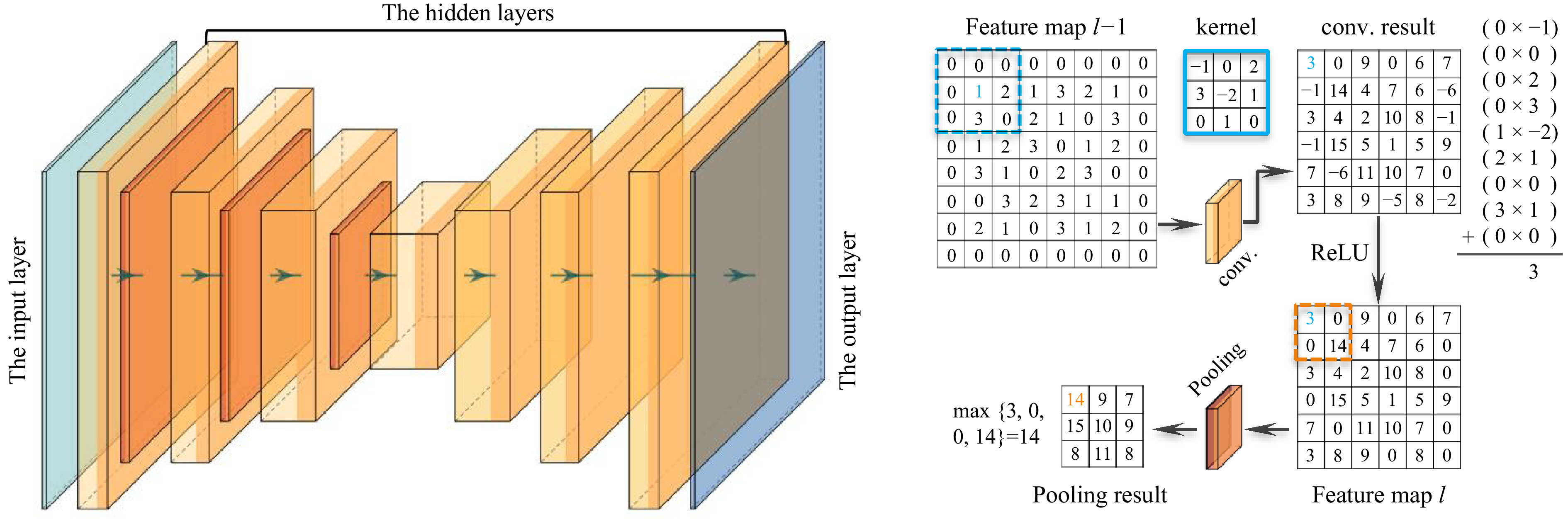

Fig. 2  A conceptual architecture of CNN.

In the feedforward NN model described by Eq. 7, the neurons in neighboring layers are typically fully connected with the weight and bias parameters independent of each other. Although DNN has been employed to solve many problems in computational imaging^117−119, ranging from ghost imaging to imaging through scatterers, there are several issues with it. First, as there are too many parameters to train, it often has the issue of overfitting. Second, it requires a large memory footprint to temporally store the parameter set $ \Theta $ and thus the training usually takes a lot of time. Third, it ignores the intrinsic structure that the data to be processed may have. This is in particular important for the tasks of speech and image processing. Images, in particular, have significant intrinsic structures. For example, neighboring pixels may have similar values; the image may be shift-invariant, etc. It is therefore highly demanded to have units in a neural network to learn these features.

Inspired by the physiological mechanism of visual cortexes¹²⁰, a convolutional neural network (CNN) also has a layered structure. Indeed, it consists of an input layer, an output layer and multiple hidden layers. But the hidden layers in CNN do not have to be fully connected. Instead, each convolutional layer in CNN has a filter called kernel function, denoted by $ w $, to convolve with the incoming data $ z $ from an upstream layer, and extract a feature map of it at a certain level of abstraction. Instead of Eq. 1, the calculated feature map $ a(i,j) $ can be mathematically written as⁴²

where $ (i,j) $ and $ (m,n) $ stand for the neurons at two neighboring layers. Equation (18) means that the elements of the kernel function, $ w(m,n) $, will apply to many neurons in the layer. In other words, all those neurons share the weighting parameters in contrast to the case of DNN that each neuron is tied to a unique weight. This parameter sharing mechanism guarantees that the network just needs to optimize a much smaller set of parameters for each layer. It is because of this reason that the requirement for memory footprint and computation efficiency can be significantly reduced in comparison to DNN⁴². Indeed, the size of the kernel function is typically from $ 3\times3 $ to $ 5\times 5 $ for many applications in holography^52,64, which is very small in comparison to that of a layer.

Note that a natural image has various features in one level of abstraction. For example, an image of a human face may contain edges with different orientations. Thus it is preferable to use multiple filters in one layer to extract all these edge orientation features, generating multiple feature maps. Usually these feature maps are arranged in a three-dimensional volume as they are to pass to a downstream layer. Denoting the width $ M $ and height $ N $ as the transverse size of each feature map, and the depth $ U $ as the number of feature maps, the value of the $ (i,j)^\mathrm{th} $ pixel in the $ t^\mathrm{th} $ feature map in the $ l^\mathrm{th} $ convolutional layer $ (l\;\geq\;2) $ can be written as

where $ b^{(l)}(t) $ is a bias term for the $ v^\mathrm{th} $ feature map in the $ l $ layer, $ u $ denotes the $ u^\mathrm{th} $ feature map in the $ (l-1)^\mathrm{th} $ layer, $ w $ is the corresponding kernel function, and $ z^{(l-1)} $ is the output from the upstream layer. One can clearly see from Eq. 19 that the convolution algorithm is actually implemented by cross-correlation in CNN, in contrast to what we are familiar with in terms of Fourier optics¹²¹. However, this does not change the resulting feature maps except their indices. We adapt this custom and call both Eq. 18 and Eq. 19 convolution.

The numerical calculation of the convolution in Eq. 19 requires moving the filter across spatial dimensions of the input data $ z^{(l-1)} $. In conventional digital image processing and numerical implementation of convolution in optics¹²², the filter is moved one pixel to the right and one pixel to the bottom at a time. In the language of deep learning, this means that the stride is equal to 1. But it is not necessary to be like this in CNN. Indeed, the stride of 2 is commonly used. More specifically, for an input image of size $ N\times N $ and a kernel of size $ M\times M $ with $ {\rm{stride}} = k $, the resulting output will be of size $ [(N-M)/k+1]\times[(N-M)/k+1] $.

The output feature maps $ a^{(l)}(i,j;t) $ are then passed through an activation function, usually the ReLU function defined by Eq. 2, to a pooling layer, which performs nonlinear down-sampling. This can be done in many ways. But the one that is most commonly used and has good performance is maxpooling¹²³, which partitions each incoming feature map into a set of non-overlapping rectangle regions by using a filter with the size of $ \kappa\;\times\;\kappa $ and outputs the maximum value of each region. Thus, the spatial size of the resulting feature map is reduced by a factor of $ \kappa $. As a consequence, the number of parameters, memory footprint and amount of computation in the network can be reduced accordingly. The reduction of network parameters will of course improve the situation of overfitting. Maxpooling also guarantees that the most significant features and their rough location relative to the other features can be passed to the downstream layer.

In a typical CNN model, the convolutional layer, the ReLU layer and the pooling layer are arranged in sequence, forming the basic building block⁴². Usually several “convolution-ReLU-pooling” blocks are arranged in cascade, each of which performs the same set of operations as described above. In the end, only the most significant features (activated features) of the input data can be retained after the data stream passes through several blocks. In the applications of image recognition¹⁰⁰ and focused distance determination in holographic reconstruction⁶², a flatten layer is usually used to reshape the three-dimensional feature volume into a one-dimensional vector, which is then sent to fully-connected layer described by Eq. 1 for further analysis. In the applications of holographic reconstruction⁵¹⁻⁵³ and aberration compensation⁵⁸, however, one wishes to reconstruct the object function and need a path to transform the activated feature maps back to the image pixels. This can be implemented by adding a deconvolutional network^124,125, which consists of a series of unpooling (reverse maxpooling), rectifying, and transpose convolution operations that upsample the feature maps many times until it reaches the size of the input hologram. The elegant U-Net¹²⁶ operates in a similar way, except that the unpooling layers are replaced by “up-convolution” layers.

A CNN model can be trained in the way as we described in Sec.. It involves the calculation of the gradient of the loss function with respect to the weight of every kernel function, which is then used to update the weight, usually according to the Adam method¹¹³. The back propagation model is a little different. One can refer to Ref. 42 for more details.

When the network goes deeper, it becomes very difficult to train because of the problems such as gradient vanishing and exploding¹²⁷. He et al. proposed the residual neural network, or ResNet for short, to address this problem¹⁰¹. The most distinguished feature of ResNet is that two distanced layers can be connected directly through the short-cut. That says, the signal goes through a series of “convolution-ReLU-convolution” blocks instead of the “convolution-ReLU-maxpooling” in CNN. The result is then added to the input of this block. Thus, the forward propagation model can be formulated as¹⁰¹

where $ f^{(l)} $ is the CNN forward propagation function defined in Eq. 19, $ {\boldsymbol{W}}^{(l-1,l)} $ is the weight that connects layer $ l-1 $ and layer $ l $. It is clearly seen that the input of layer $ l-2 $, $ {\boldsymbol{z}}^{(l-2)} $, is directly connected to the $ l^\mathrm{th} $ layer. As it does not need to undergo the nonlinear transform, the gradient will flow easily during back propagation.

Nowadays, a common and practical strategy to design a DNN to solve holographic problems is to take U-Net as a backbone, and incorporate into it the ResNet ingredient of short-cuts^{53,55,58,71,128−130}. The U-Net architecture can also be extended to allow the extraction of features of different size by introducing multiple channels in the down-sampling convolutional blocks^{51,52,59,131−133}. Another interesting extension of U-Net is the so-called U-Net++¹³⁴, which has a pyramid shape architecture. It essentially consists of an encoder and a decoder that are connected through a series of nested, dense skip pathways, bridging the semantic gap between the feature maps of the encoder and the decoder prior to fusion¹³⁵.

Generative adversarial networks (GAN's) are NN's that learn to generate synthetic instances of data with the same statistical characteristics as the training data¹³⁶. GAN is able to keep a parameter count significantly smaller than other methods with respect to the amount of data used to train the network. It the field of holography, GAN has been used for wavefront reconstruction^67,137,138, enhancement¹³⁹ and image classification¹⁴⁰. It can be trained on paired data¹³⁹, unpaired data^67,138 or even unsupervisely¹⁴⁰ in some cases.

Architecturally, GAN is constituted of two neural networks, one of which is called the generator, and the other, the discriminator. As shown in Fig. 3, the two networks are pitted one against the other (and thus “adversarial”) in order to generate new, synthetic instances of data that can pass for real data. Explicitly, the generator G is a deconvolutional neural network^124,125 that generates new images as real as possible from a given noise variable input $ z $, whereas the discriminator D is a CNN-based classifier that estimates the probability of a generated image and determines if it looks like a real image from the training set or not.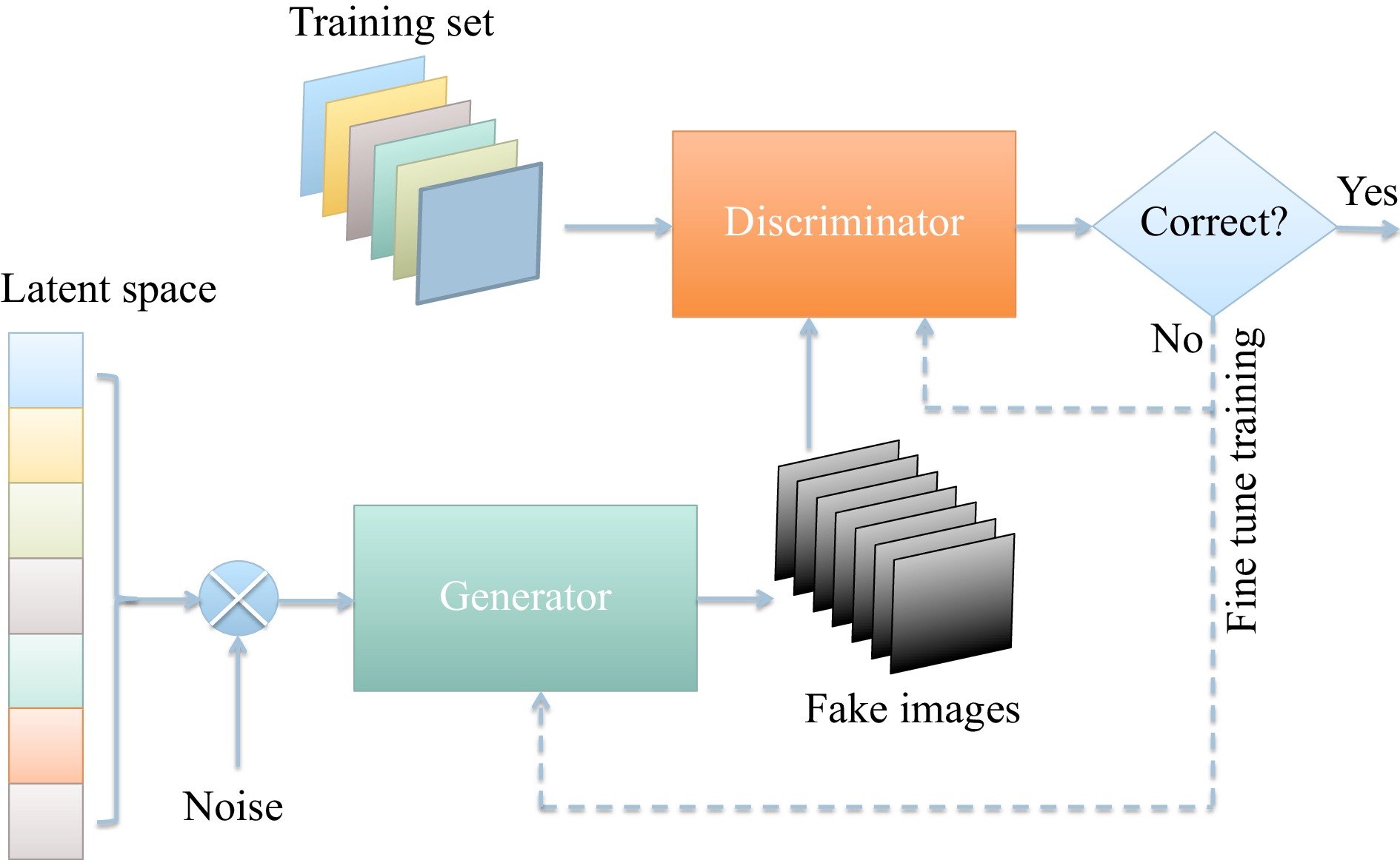

Fig. 3  A conceptual architecture of GAN.

To proceed, let us denote the probability distribution of the input variable $ z $ as $ p_z $, that of the generator over data $ x $ as $ p_g $, and that of the discriminator over real sample $ x $ as $ p_r $. The purpose of GAN is to make sure that the discriminator's decisions over the real data are accurate by maximizing $ \mathbb{E}_{x \sim p_{r}(x)} [\log D(x)] $, while the discriminator outputs a probability $ D(G(z)) $ that is close to zero by maximizing $ \mathbb{E}_{z \sim p_{z}(z)} [\log (1 -D(G(z)))] $ for a given generative data instance $ G(z) $, where $ z \sim p_z(z) $.

Thus, one can see that D and G are actually playing a minimax game so that the objective is to optimize the following loss function¹³⁶

where

Note that for any $ (a, b) \in \mathbb{R}_2 \backslash\{0, 0\} $, the function $ y \rightarrow a \log(y) + b \log(1-y) $ achieves its maximum in $ [0, 1] $ at $ y = {a}/({a+b}) $. It is then straightforward to obtain the best value of the discriminator¹³⁶

Once the generator is trained to its optimal, $ p_g = p_{r} $. Thus $ D^*(x) = 1/2 $, and the loss function $ {\cal{L}}(G, D^*) = $$ -2\log2 $.

GAN can be trained by using SGD-like algorithm such as Adam¹¹³ as in the case of CNN. But the discriminator and the generator should be trained against a static adversary¹⁴¹. That is, one should hold the generator values constant while training the discriminator, and vice versa.

There are several adaptations of GAN, among which the cycle-GAN¹⁴² and conditional GAN (cGAN)¹⁴³ have been adopted for holography. Different from GAN, the purpose of the generator in cycle-GAN is not to generate an image from noise, but to take a hologram as its input and extract the most significant features via a series of convolutional layers, and then build a reconstructed image of the same size as the input hologram from these transformed features using a series of transpose convolutional layers. The most distinguished idea behind cycle-GAN is the introduction of a cycle consistency loss

that imposes a constrain to the model. The generator $ G $ generates an object image $ x $ from a hologram $ z $, and $ F $ generates the hologram $ z $ of $ x $. Thus, the total loss function can be defined as

where $ D_x $ and $ D_z $ are the discriminators of $ x $ and $ z $, respectively, and $ {\cal{L}}_{{\rm{GAN}}_x}(G,D_x,x,z) $ and $ {\cal{L}}_{{\rm{GAN}}_z}(G,D_z,x,z) $, defined by Eq. 22, are the conventional GAN loss of the objects $ x $ and holograms $ z $ in the training set. It is clearly seen that $ x $ and $ z $ show up independently in each term of $ {\cal{L}}(G,F,D_x,D_z) $, meaning that they do not need to pair up in the training set.

The training of DNN usually requires a large set of data, the size of which is typically ranging from a few thousands to tens of thousands in a typical proof-of-concept demonstration. The amount of labeled data is far less than that is used for deep learning applications in other communities such as computer vision. For example, AlexNet¹⁰⁰ was trained on a set composed of $ 1.2 $ million images.

In the case of supervised training the data used for training should be labeled so that every input data $ {\boldsymbol{x}}_k $ is paired up with a corresponding ground truth data $ {\boldsymbol{y}}_k $. But it is not necessary to do so in some other cases^67,140 like unsupervised training. Optical acquisition of these data usually takes the most time, and requires the optical instruments in use to be stable during the long period. Otherwise, the data pairs cannot be registered well enough to match each other⁵¹. However, since holography is extremely sensitive to environment vibration¹⁰, it is unavoidable to capture such vibration in the holograms during the time of acquisition (usually tens of hours depending on the number of holograms required to train the DNN), resulting in the instability of the fringe patterns. However, we have shown that DNN can be well trained on these “noisy” data⁵².

An alternative and more flexible way to generate the training data is to use a numerical simulator provided that the physical system that describes the data link from the source to the detector can be accurately modeled. For example, this strategy has been applied to phase unwrapping⁷² as well as speckle removal^66,68, ghost imaging¹³¹, STORM^144,145 and diffraction tomography¹⁴⁶.

The raw data are mainly taken from MNIST¹⁴⁷, Faces-LFW¹⁴⁸ and CelebAMask-HQ¹⁴⁹, which are publicly available. In most of the proof-of-concept experiments, a spatial light modulator (SLM) is used to display these images in order to form the holograms of them by using a standard holographic system. However, in most of the practical applications of holography, it is not the 2D hand-written digits, English letters¹⁴⁷, or 2D human faces^148,149 that are of interest. Thus, DNN trained on these data sets is difficult to be generalized¹⁵⁰ to cope with most of the objects in the real world.

Recently, Ulyanov et al. have shown that the structure of a generator network can capture a great deal of low-level image statistics prior to any learning¹⁵¹. This can be generalized to a more general DNN such as the U-Net by incorporating a physical model into it, resulting in an untrained neural network that does not require any data to train⁵⁵. It can be used to reconstruct the holograms of realistic objects. Indeed, over the past year, untrained DNN has been applied by to solve problems of holographic reconstruction⁵⁵⁻⁵⁷, phase unwrapping⁷³, phase microscopy¹⁵², diffraction tomography¹⁵³ and imaging¹⁵⁴, and even ghost imaging¹⁵⁵. I will discuss it in more detail later on.

So far I have introduced several important DNN models that are widely used in optics and holography. Indeed, DNN has been shown to outperform conventional physics-based approaches. For example, DNN allows twin-image-free reconstruction from a single-shot in-line digital holography⁵². A major reason for the success is that DNN, given enough data, can learn feature hierarchies with features from higher levels of the hierarchy formed by the composition of lower level features¹⁵⁶ even explicit formulation of a system's exact physical nature is impossible owing to its complexity^119,132.

However, it is also well-known that DNN has a black-box issue¹⁵⁷: the information stored in DNN is represented by a set of weights and connections that provides no direct clues to how the task is performed or what the relationship is between inputs and outputs¹⁵⁸. When it is used to solve real-world physical problems, DNN has met with limited success due to a number of reasons: First, DNN requires a large amount of labeled data for training, which is rarely available in real application settings¹⁵⁹. As discussed above, for most of the leaning-based methods for optical imaging and holography, an SLM is required to display the ground-truths. Frequently, the publicly available dataset such as the MNIST¹⁴⁷ database is used for demonstration. But this is hard to generalize to real-world samples owing to the issue that DNN models can only capture relationships in the available training data¹⁵⁰. Second, DNN models often produce physically inconsistent results¹⁶⁰ when violating fundamental constraints. Third, the output is unexplainable¹⁶¹.

Thus, it is highly desirable to take the benefits of both DNN models and physics models, and develop physics-informed or physics-guided DNN^162−165. Barbastathis and coworkers⁴⁵ have concluded three different ways to incorporate a physical model into DNN, namely, recurrent physics-informed DNN, cascaded physics-informed DNN, and single-pass physics-informed DNN. In contrast, Ba and coworkers have concluded four different ways¹⁶⁶: physical fusion, residual physics, physical regularization, and embedded physics. One can see that both these two ways of classification are somewhat equivalent.

According to Ba et al.¹⁶⁶, physical fusion is the most straightforward way. It feeds directly the solution from a physics model as (part of) the input to a DNN model. Barbastathis and coworkers⁴⁵ term this method as single-pass physics-informed DNN. This strategy has been employed in the very first work on learning-based holographic reconstruction, in which Rivenson et al.⁵¹ used a conventional diffraction-based algorithm⁵ to reconstruct a blurred wavefront from a hologram, and then used a trained DNN to improve the quality. This method has also been used for other problems such as ghost imaging¹¹⁷ and phase retrieval¹⁶⁷.

In contrast, residual physics is to add the physical solution to the DNN output so that the DNN model only needs to learn the mismatch between the model-based solution and the ground truth¹⁶⁸. Physical regularization, on the other hand, harnesses the regularization term from a set of physical constraints to penalize the network solutions. The regularization term can be appended as part of the loss function explicitly or through a reconstruction process from physics¹⁶⁰. These two concepts are similar to the recurrent physics-informed DNN and cascaded physics-informed DNN discussed in⁴⁵.

More exciting is the strategy of embedded physics. As shown in Fig. 4, the central idea is to take the physical model inside the network optimization loop: the physical model takes care of the well-posed forward propagation while DNN, the ill-posed backward propagation, in each iteration^{55−57,138,152−155}. The error between the forward calculated output and the measured data can be used to estimate a defined loss function, which is then used to update the weights based on an SGD-like algorithm.

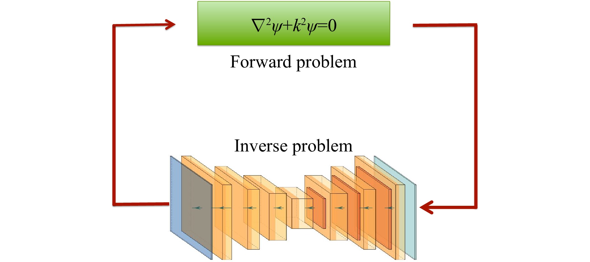
Fig. 4  A typical architecture of an embedded physics DNN.

Here I would also like to draw the attention of the readers to an emerging strategy, which I call network approximating physics. By the name, it is to approximate a physical model by using a DNN^78,169. For example, Shi et al. proposed to approximate the Fresnel zone plates through successive application of a set of learned $ 3\; \times\; 3 $ convolution kernels⁷⁸ in order to build a DNN model that can approximate the Fresnel diffraction and occlusion.

After the brief introduction of deep learning neural networks in Sec. 1, now I will review some of the recent studies on the applications of deep learning in holography in this section. Before going into the detail, it is worthy of mentioning that the idea of using NN to for holography is not new. It has been proposed and demonstrated many years ago^170−174. But the performance of neural networks was limited at that time because they were not deep enough due to the limited computation power. Indeed, one can find that some of the ideas demonstrated recently have been proposed at that time.

A hologram can be formed by the superposition of the object beam $ u_o(x,y) $ that carries the information of an object of interest and a reference beam $ u_r(x,y) $, where $ (x,y) $ is the spatial coordinates in the hologram plane

where the symbol * stands for phase conjugate.

Intuitive approaches for holographic reconstruction are based on the physical model of diffraction, i.e., the numerical calculation of the diffraction process of the wave field⁶. In the off-axis geometry with a sufficient high carrier frequency all the three terms in Eq. 26 are well separated in the Fourier space, and therefore one can simply apply a spatial filter to remove the two unwanted terms. However, spatial filtering inevitably results in the loss of high-frequency components, which greatly hinder the reconstructed image quality³². In addition, one can use only a small part of the spatial bandwidth product (SBP) that the camera can offer^175−177 in this case. In in-line DH the reconstructed image are overlapped with the twin-image and the zeroth-order terms. Since the removal of the zeroth-order is comparatively straightforward, most of the studies on in-line holographic reconstruction is to deal with the twin image term.

Physics-based approach relies on some physical models as suggested by the name. Back in 1951, Bragg and Rogers¹³ had realized that the twin image is actually the out-of-focus copy of the reconstructed object image, and it can be eliminated by the subtraction of the defocused wavefront from the other. But this method is technically tricky, and can be implemented only after the invention of DH^178,179. The most widely used strategy nowadays is to tune some physical parameters of the optical system and acquire the corresponding holograms so as to set up a small linear equation system that relates the recorded holograms and the tuning parameters and solve for the object wavefront. For example, one can introduce multiple phase retardations stepwise in the reference beam and acquire the phase-shifted holograms²⁰⁻²², or move the camera along the propagation direction²³⁻²⁵, or slightly tune the wavelength of the illumination laser beam²⁶. However, as the control of these parameters is extremely difficult for very short wavelength radiation, these methods are infeasible for electron holography¹⁸⁰, X-ray holography¹⁸¹, or $ \gamma $–ray holography¹⁸². In this case, one should implement the phase shift by using an amplitude element such as the Chinese Taiji lens¹⁸³ or the Greek-ladder zone plate¹⁸⁴.

Mathematically, the twin image artifact arises due to the missing of the phase when the hologram is recorded¹⁸⁵. This suggests that the twin image artifact can be resolved if the missing phase of the hologram $ |u_0(x,y)+u_r(x,y)| $ can be retrieved. This is the fundamental logic behind the phase-retrieval approach. Effectively, phase retrieval can be solved by using either a deterministic algorithm that is called now the transport-of-intensity equation (TIE)¹⁸⁶, or an iterative algorithm such as the Gerchberg-Saxton (GS)²⁷ and/or the Hybrid-Input-Output (HIO) algorithm²⁸. This is in particular useful when the coherence of radiation source in used is poor (X-ray, for example). Thus the communities of X-ray holography and electron holography have made intensive studies since the late 1980s^{185,187−190}. Along with the improvement of the technique and better modeling of the objective function, people now can achieve the reconstruction of the whole wavefront²⁹⁻³¹.

Phase retrieval is actually an inverse source problem of image reconstruction from magnitude^191,192. It can be formulated as a more general class of inverse problems. The inverse problem approach treats the DH image reconstruction as a pure digital signal processing (DSP) problem, and solves it by using various numerical algorithms, such as statistical model^32,33, sparsity-enforcing prior³⁴, least squares³⁵, regularization^36,37, and compressive sensing³⁸⁻⁴⁰. A critical issue with it, from the computational point of view, is that the two-dimensional (2D) hologram must be rearranged as a one-dimensional (1D) vector in contrast to treating it as a 2D array in the two other aforementioned approaches. It thus requires the calculation of very large matrices, which is too heavy to do efficiently¹⁹³.

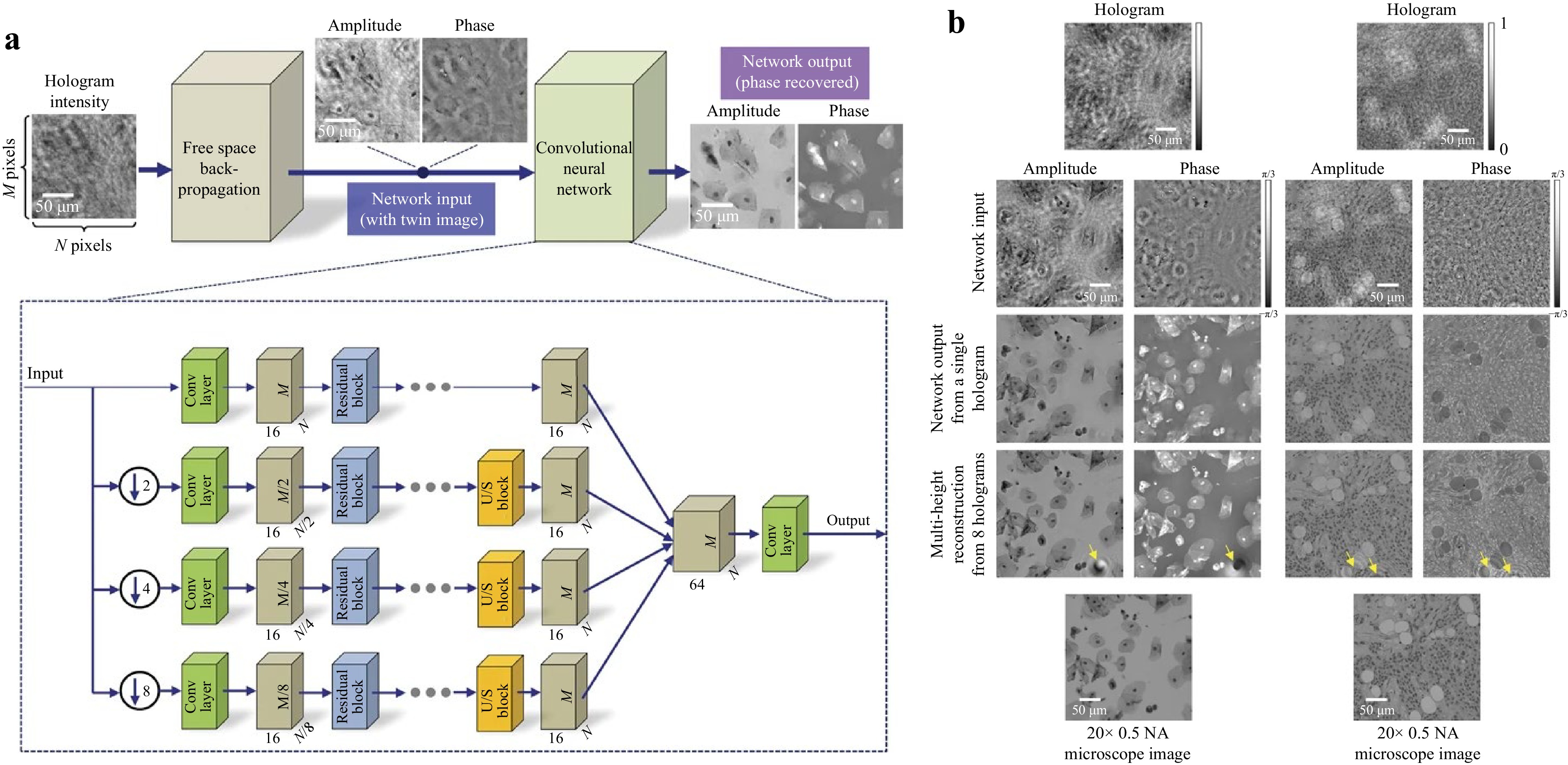
Several strategies have been proposed to solve the problem of holographic reconstruction. The most straightforward approach is the end-to-end DNN^52,54. For example, Wang et al.⁵² took the advantages of ResNet¹⁰¹ and U-Net¹²⁶, and developed an alternative approach called eHoloNet for end-to-end holographic reconstruction. eHoloNet receives the raw digital hologram as the input, and produces the artifact-free object wavefront, which is a phase profile in their study, as the output. They treat the holographic reconstruction as solving an ill-posed inverse problem for the function $ {\cal{R}} $ that maps directly the hologram space to the object space

where $ \theta $ is an explicit setting of the network parameters $ \Theta $, $ {\cal{L}}(\cdot) $ is the loss function to measure the error between the $ n^\mathrm{th} $ phase object $ u_{o,n} $, and the corresponding in-line hologram $ {\cal{R}}_\theta\{I_n\} $, and $ \Psi(\theta) $ is a regularizer on the parameters with the aim of avoiding overfitting¹⁹⁴. They demonstrated their approach using 10,000 handcraft images from the MNIST dataset¹⁴⁷ and 12,651 images of the USAF resolution chart. All these images were resized to $ 768\;\times\;768 $ pixels and displayed on a phase-only SLM (Holoeye, LETO), making them effectively phase objects. The in-line digital holograms of all the 22,651 phase objects were acquired by a Michelson interferometer. 9000 pairs of handcraft images and their holograms and 11,623 pairs of resolution charts and their holograms were used to train the eHoloNet, respectively. The lefts were used for test.

In order to reconstruct both the intensity and phase simultaneously from a single digital hologram, Wang et al. proposed a Y-shaped architecture⁵⁴. The loss function then is defined as

where $ {\cal{L}}_I $ and $ {\cal{L}}_P $, defined according to Eq. 15, denote the loss function of the intensity and phase of the complex wavefront, and the weight $ \lambda\; =\; 0.01 $ in their experiments so as to enforce the significance of the phase.

The end-to-end approach can be implemented via GAN^67,137 as well. One advantage to use GAN is that the training data do not need to pair up.

The second approach is the physics fusion or single-pass physics-informed DNN^51,53. As discussed in Sec., this is a two-step process. First, the complex wavefront was reconstructed by using the conventional numerical free space propagation back to the object plane. As aforementioned, the reconstructed wavefront is usually overlapped with the twin image, and the zeroth-order artifacts. The amplitude and phase of the reconstructed wavefront were then sent separately into a DNN, which has been trained to remove all these artifacts⁵¹. In their study, Rivenson et al. adopted a network architecture based on ResNet¹⁰¹, as shown in Fig. 5a. The network was trained by the directly reconstructed amplitude and phase using numerical free space propagation algorithm and the corresponding ground truths (which are reconstructed by using phase retrieval algorithms from multiple holograms^195,196). 100 image pairs were used to train the network. The results are shown in Fig. 5b. This method can be applied to off-axis DH to improve the quality of the reconstructed image as well⁵³.

Fig. 5  a The DNN architecture and the pipeline for holographic reconstruction proposed by Rivenson et al.51 and b the experimental results. (adapted from 51).

The third one, physics-informed DNN is an exciting approach for holographic reconstruction. For example, Wang et al. have proposed a physics-enhanced DNN (PhysenNet)⁵⁵ that employs a strategy of incorporating a physical imaging model into a conventional DNN. PhysenNet has two apparent advantages. First, it does not need any data to pre-train. This can be clearly seen in the objective function

where $ I $ is the hologram or intensity pattern from which we wish to reconstruct the phase, and $ H $ is the physical model, which is the Fresnel transform in their explicit case. It can be any other image formation process that can be accurately modeled^{55−57,73,152−155}. Eq. 29 suggests that PhysenNet just requires the data to be process ($ I $ in this case) as its input. The interplay between the physical model and the randomly initialized DNN provides a mechanism to optimize the network parameters, and produce a good reconstruction. Second, the reconstructed image satisfies the constraint imposed by the physical model so that it is interpretable¹⁶³. The experimental results are plotted in Fig. 6.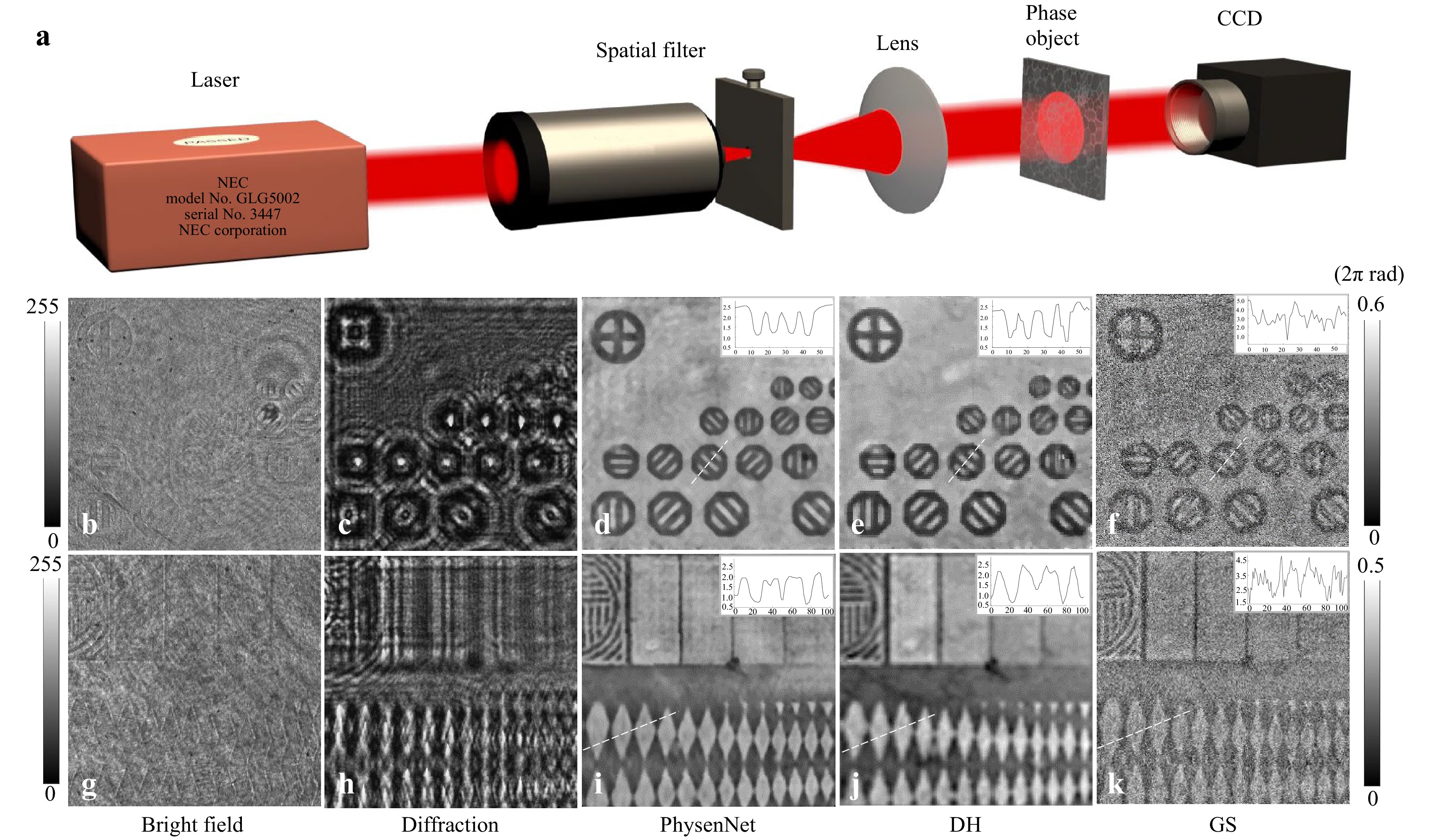

Fig. 6  Experimental results. a Experimental set-up. b and g show two different parts of the phase object, c and h show the diffraction patterns, d and i show the phase images reconstructed by PhysenNet, e and j show the phase images reconstructed via off-axis digital holography, and f and k show the phase images reconstructed with the GS algorithm. (after 55).

The DNN model in PhysenNet can be replaced by other neural networks dependent on the task in hand. For example, Zhang et al. have demonstrated the incorporation of a phase imaging model into GAN¹³⁸.

Holographically reconstructed phases are usually wrapped owing to the $ 2\pi $-phase ambiguities and thus need unwrapping, which is also a typical ill-posed inverse problem. Conventional phase unwrapping techniques estimate the phase either by integrating through the confined path (referred to as path-dependent methods) or by minimizing the energy function between the wrapped phase and the approximated true phase (referred to as minimum-norm approaches)⁷². DNN provides a very feasible solution to this kind of problem because it can resolve the issues such as error accumulation, high computational time and noise sensitivity that conventional techniques frequently encounter.

Actually, the idea of using neural networks for phase unwrapping has been proposed by Takeda et al.¹⁷¹ and Kreis et al.^172,173 in the 1990s. But with the developments of DNN techniques and computer power, much deeper neural networks are available now. There are ways to treat the phase unwrapping problem from the DNN point of view. A straightforward way is to take it as a regression problem, and develop a DNN to map a wrapped phase to an unwrapped phase. This can be done, for example, by using a U-Net trained on labeled data⁷¹. One research line is to improve the network design, aiming to enhance the phase quality. For example, Zhang et al.¹⁹⁸ have proposed a DNN model called DeepLabV3+, which can achieve noise suppression and strong feature representation capabilities. They demonstrated that it is out-performed the conventional path-dependent and minimum-norm algorithms. It is also possible to unwrap a phase by using an untrained DNN in a way similar to PhysenNet⁵⁵. For example, Yang et al. have experimentally demonstrated that the proposed method faithfully recovers the phase of complex samples on both real and simulated data⁷³.

Alternatively, one can treat phase unwrapping as a classification problem. For example, Zhang et al.¹⁹⁷ have demonstrated it by transferring phase unwrapping into a multi-class classification problem and introduced an efficient segmentation network to identify the classes. Their experimental results are plotted in Fig. 7.

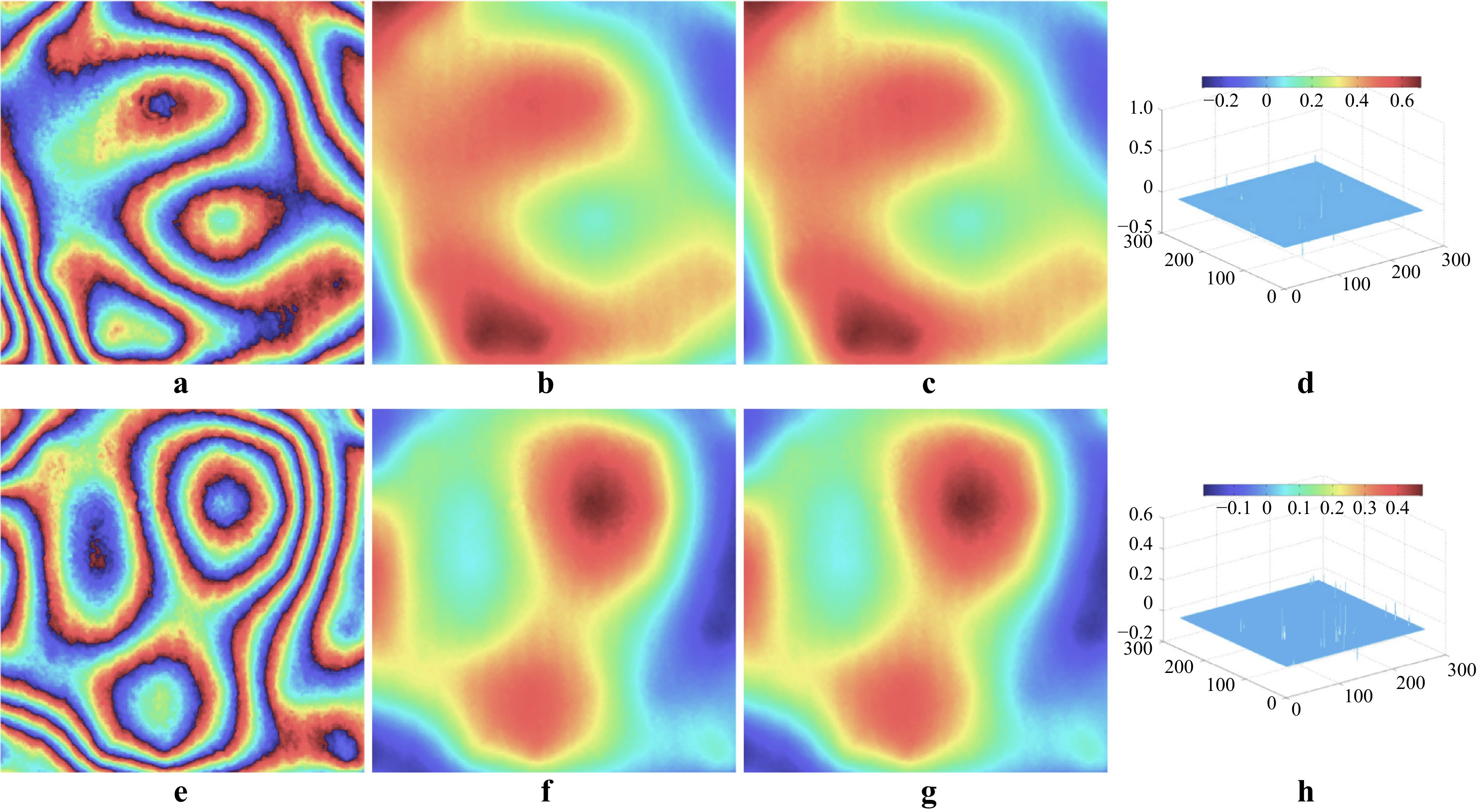
Fig. 7  Unwrapping results on real data. From left to right are: wrapped phases [input, a, e], reconstructed unwrapped phases by the DNN [b, f] and MG [c, g], and differences [d, h]. (after 197).

Learning-based phase unwrapping algorithms have been applied to solve the problems in many different fields of studies, such as biology¹⁹⁹ and Fourier domain Doppler optical coherence tomography²⁰⁰.

Autofocusing is about the automatic determination of the numerical calculation of the free space propagation distance of the wavefront from the hologram plane²⁰¹. This is in particular important for the applications of DH in industrial and biological inspection²⁰². Conventionally, the focused distance is determined by a criterion function with respect to the reconstruction distance. The criterion function can be defined in many ways, such as the entropy of the reconstructed image, the magnitude differential²⁰¹, and sparsity²⁰³, and usually has a local maximum or minimum value at the focal plane.

Learning-based autofocusing algorithms employ different strategies. The prediction of the focusing distance is not made by searching a local extreme value of a criterion function, but by directly analyzing a digital hologram by using a deep neural network. One can think of autofocusing as a regression problem or a classification problem. The regression approach is to train the network by using a stack of artifact-free reconstructed images that are paired up with a hologram⁵⁹⁻⁶¹. Each image in the stack is associated with a number that indicates the reconstruction distance. All these numbers are used to rectify the output layer during the training process. Taking the advantage of the U-Net¹²⁶ and ResNet¹⁰¹, Wu et al⁶⁵ proposed the HIDEF (Holographic Imaging using Deep learning for Extended Focus) CNN. This allows the direct reconstruction at the correct distance when a hologram is inputted to the trained HIDEF CNN. Jaferzadeh et al. proposed a DNN model with a regression layer as the top layer to estimate the best reconstruction distance²⁰⁴.

The classification approach was proposed by Ren et al⁶² and Shimobaba et al⁶³. For example Ren and coworkers experimentally recorded the 5000 holograms of several objects (a resolution chart, a testis slice, a ligneous dicotyledonous stems, an earthworm crosscut, etc.) at 10 different distances; and use the holograms and the associated distance values to train their neural network.

An alternative strategy is to take the focusing distance as an uncertain parameter, and ask the neural network to optimize automatically¹³⁵. In this case, the objective function can be written as

where the uncertain focusing distance $ d $ enters the the physical model $ H $ now, and will be optimized by the network.

The objective function in the form of Eq. 30 is similar to Eq. 29. This suggests that the only input required by the neural network is the hologram $ I $, and the DNN does not need to be pre-trained on any dataset. As shown in Fig. 8, the algorithm will converge to the exact distance value along with proceeding of the iteration.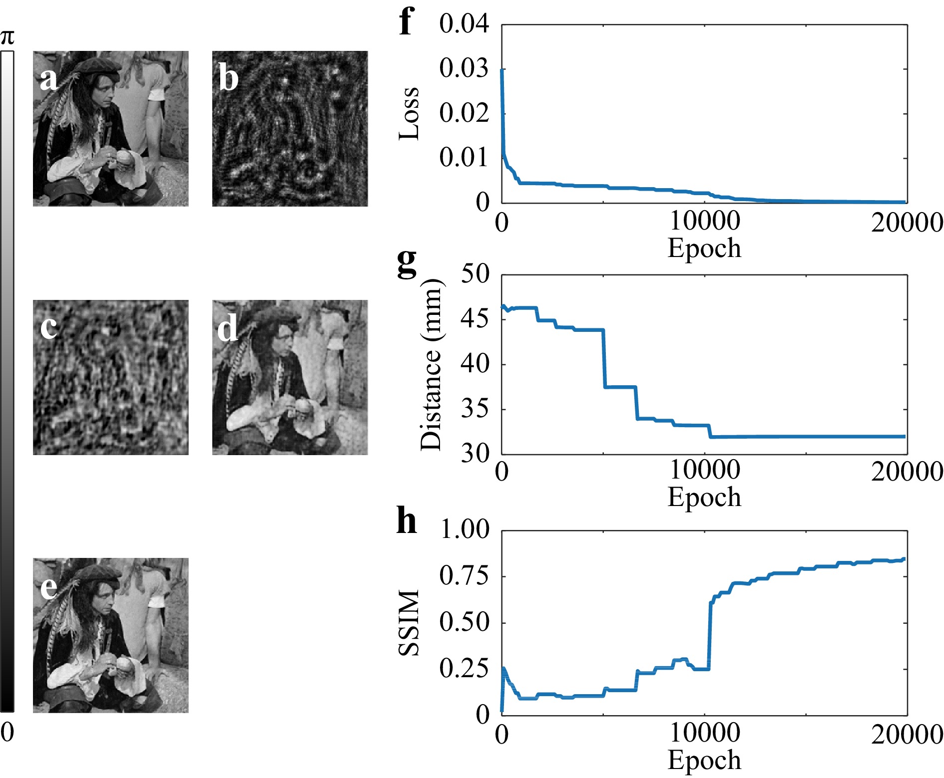

Fig. 8  The reconstruction process of a phase object. a the original phase object. b the diffraction pattern. The retrieved phase at the epoch of c 900, d 10300, and e 19800. The behavior of f the loss function, g estimated distance, and h the SSIM value as a function of the number of epoch. (after 135).

Learning-based approaches have also been used for phase aberration compensation in digital holographic microscopy^58,152,205. Again, phase aberration compensation can be formulated as a classification⁵⁸ or a regression^152,205 problem. In the work by Nguyen et al.⁵⁸, the role DNN plays is to segment the reconstructed and unwrapped phase. The phase aberration then can be determined by Zernike polynomial fitting, and its conjugate can be numerically calculated to compensate the aberration. Nguyen et al. experimentally took the holograms of 306 breast cancer cells as the input and the corresponding manually segmented maps as the output to train their neural network, which is also a U-Net + ResNet architecture in this case. They used the softmax function defined in Eq. 6 in the last layer in their neural network to calculate the prediction probability of background/cell potential, and the cross-entropy loss defined in Eq. 17 for back propagation. The experimental results are plotted in Fig. 9.

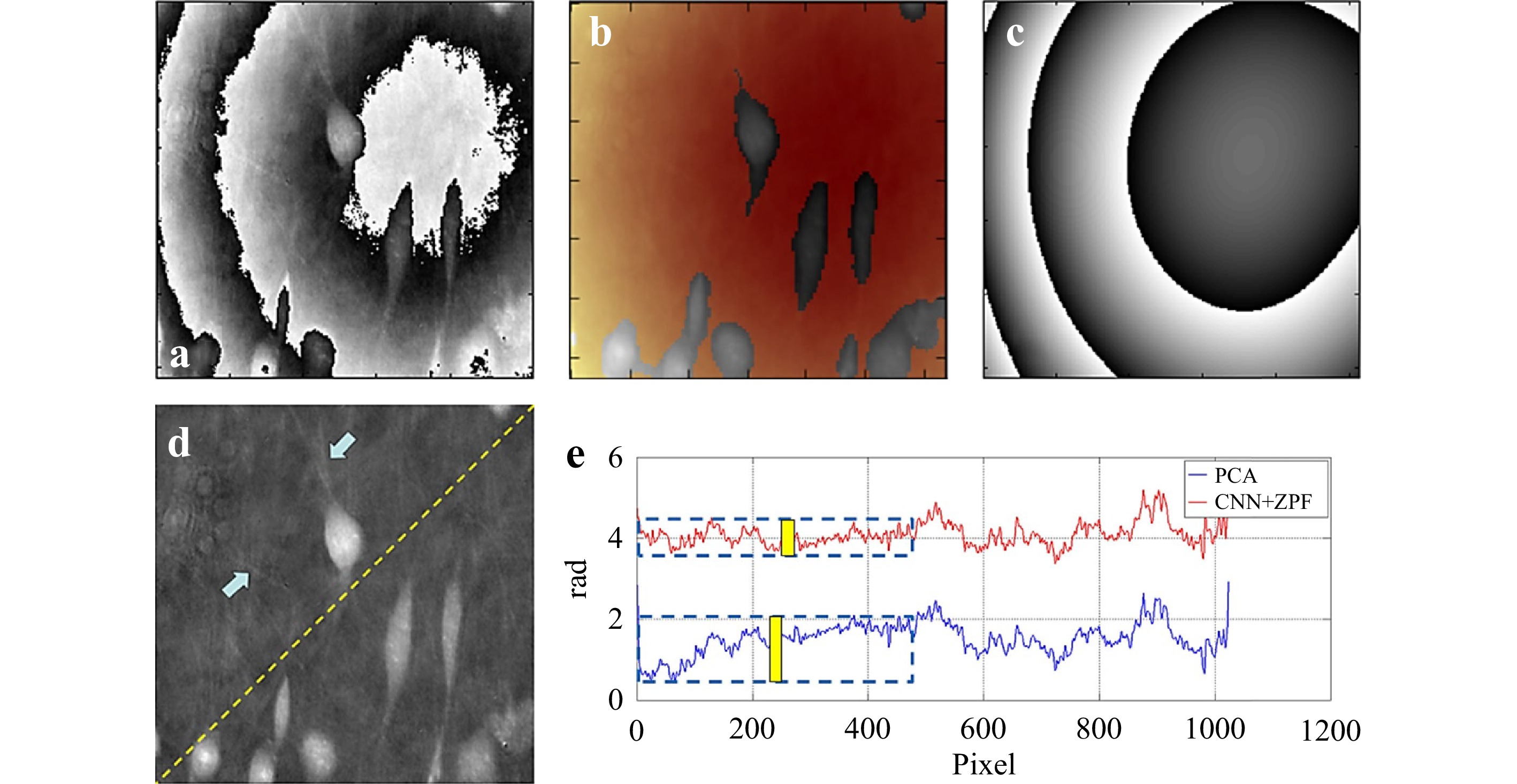
Fig. 9  a Phase aberration, b unwrapped phase overlaid with CNN’s image segmentation mask, where background (color denoted) is fed into ZPF, c conjugated residual phase using CNN + ZPF, d fibers are visible after aberration compensation and are indicated by blue arrows, and e phase profile along the dash line in d. Yellow bars denote the flatness of region of interest. (after 58).

In contrast, the regression approach proposed by Xiao et al.²⁰⁵ endeavors to optimize the coefficients for constructing the phase aberration map that act as responses corresponding to the input aberrated phase image. Embedded physics DNN can be used for this problem as well. Encapsulating the image prior and the system physics, Bostan et al.¹⁵² have proposed an untrained DNN that can simultaneously reconstruct the phase and pupil-plane aberrations by fitting the weights of the network to the captured images.

As a coherent imaging modality, DH reconstruction is also influenced by the coherence of the illumination laser source^11,206, which naturally results in speckle²⁰⁷. The elimination of speckle noise has been one of the main issues in DH. Conventionally, this can be done either optically or digitally. Optical methods usually require multiple measurements under different conditions. Digital methods can work on a single hologram but the reduction of speckle results in the loss of information as well. Bianco et al have given a very nice review of the most important speckle removal techniques²⁰⁸.

Recently, Jeon et al.⁶⁶ have demonstrated that, by using DNN, it is possible to remove the speckle without any degradation of the image quality. The network architecture they used is again the combination of U-Net and ResNet. For supervised learning, one needs to pair up the speckled images and the corresponding speckle-free ones in order to train the network. But speckle-free images are unlikely to be obtainable from experimentally acquired holograms. So they used numerically generated speckled images from speckle-free images according to the model $ {\boldsymbol{y}} = {\cal{R}}({\boldsymbol{x}})+ $$ {\cal{N}}(0,\varsigma^2) $, where $ {\cal{R}}(\varsigma) $ is the Rayleigh distribution with scale parameter $ \varsigma $, and $ {\cal{N}}(\mu,\varsigma^2) $ is the Gaussian distribution with the mean $ \mu $ and standard deviation $ \varsigma $, to train their network, and test it with experimentally acquired holograms. Similar DNN can be applied to remove the speckle noise in phase image from holographic interferometry^68,69. The strict requirement of labeled data can be released by using a more suitable network architecture such as Noise2Noise²⁰⁹. For example, Yin et al.²¹⁰ have demonstrated a speckle removal DNN without using clean data.

CGH has been recognized as the most promising true-3D display technology since it can account for all human visual cues such as stereopsis and eye focusing^8,9,88,89 as well as a powerful tool for the test of optical elements⁸⁴⁻⁸⁶. In particular, for the application in holographic display, it requires the generated holograms to be reasonably large in size. But the calculation of such holograms within acceptable time has been one of the main challenges in this field²¹¹. Although iterative phase-retrieval algorithms^27,28,87,212 have been intensively employed for this task, modern approaches for CGH calculation are non-iterative^{88,89,211,213}, in combination of acceleration techniques such as look-up table^90,214 and the use of GPU²¹⁵.

The use of DNN has dramatically accelerated the calculation of CGH^{74−76,78−81}. People have used U-Net-based architecture to generate phase-only holograms⁷⁴ and binary holograms²¹⁶, Y-shaped architecture to generate multi-depth holograms⁷⁶, and autoencoder-based DNN for the fast generation of high-resolution holograms^80,81. DNN has also been used to improve the quality of holographic display²¹⁷, and it allows to train in the loop⁷⁷. Eybposh et al. have demonstrated an unsupervised learning based on GAN to achieve a fast hologram computation⁷⁵, although there is argument that this indirect training strategy may not obtain an optimal hologram⁸¹. The superb DNN-based algorithms allow the design of CGH to generate not just scalar but even arbitrary 3D vectorial fields in an instant and accurate manner²¹⁸.

A DNN-based CGH synthesis technique called tensor holography for true 3D holographic display has been proposed recently by Shi et al.⁷⁸. Tensor holography is a physics-informed DNN technique. It imposes underlying physics (Fresnel diffraction) to train a CNN as an efficient proxy for both. Tensor holography was trained on MIT-CGH-4K Fresnel holograms dataset, consisting of 4000 pairs of RGB-depth (RGB-D) images and the corresponding 3D holograms that take the occlusion effect into account. Thus their DNN takes the 4-channel RGB-D image as its input, and predicts a color hologram as a 6-channel image (RGB amplitude and RGB phase), which can be used to drive three optically combined SLMs or one SLM in a time-multiplexed manner to achieve full-color holographic display.

Holography has been one of the important avenues to implement optical neural networks (ONN). Early researches include the optical implementations of fully-connected neural networks⁹³⁻⁹⁷ and the Hopfield model^91,92, which is the base of the recurrent neural network (RNN). Rather than using logical neurons as in the digital counterpart, holographic neural networks rely on interconnection²¹⁹ that a hologram is inherently capable of^96,97. In a fully-connected holographic neural network, the weights are stored in the pixels (neurons) of the holograms. Each neuron in a layer (hologram) performs a simple modulation of the light that impinges onto it from an upstream layer and subsequently illuminates a downstream layer. A holographic neural networks can be created in a photorefractive crystal^93,94, which is inherently a 3D device that has a potential to store billions of weights. Thus it is in principle promising to solve large-scale inverse problems. However, interest in further developments has been on the wane owing to some unfortunate reasons²²⁰.

Modern implementation of holographic neural networks takes the advantage of diffraction⁹⁸, and thus named diffraction deep neural networks (D²NN). In the hardware implementation, the holograms in D²NN are actually diffractive optical elements (DOE), which can be fabricated using 3D printing (see Fig. 10)⁹⁸, nanomanufacturing²²¹, or electric addressable digital micro-mirror devices (DMD)²²². The weights are stored in the pixels as in conventional holographic neural networks⁹³⁻⁹⁷. There are good reasons to implement D²NN on DMD and SLM: it allows the creation of parallel and reconfigurable network connections as well as the addition of nonlinearity to each layer via fast square-law detection. Such cascaded nonlinear operations strongly amplify the dimensionality of data representation so that they can leverage for challenging computations²²².

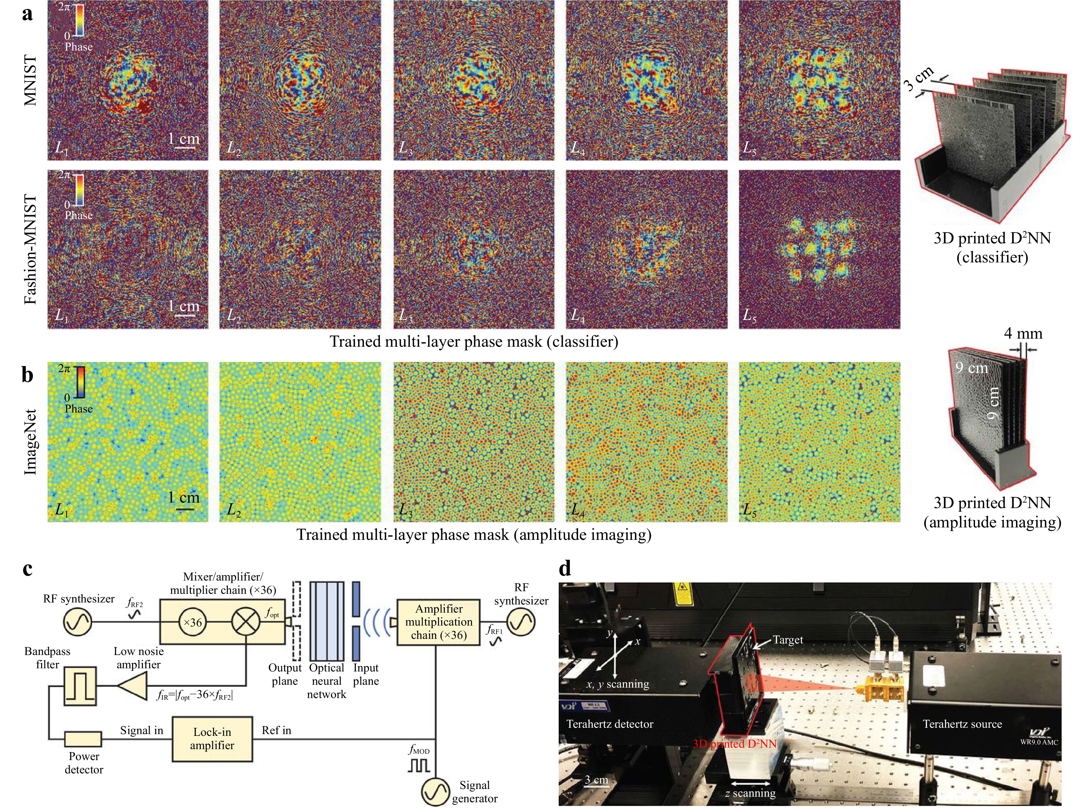
Fig. 10  Experimental testing of a 3D-printed D²NN. The optimized phase maps of five different layers of the MNIST classifier, fashion product classifier, and b the amplitude imager. Schematic c and photo d of the experimental terahertz setup. (after 98).

As many other optical neural networks²²⁰, the original D²NN engine was trained off-line⁹⁸. But efforts have been made to implement better training strategy. For example, Zhou et al. have demonstrated an in situ back propagation training²²³, Xiao et al. have proposed a back propagation technique that updates the unitary weights through the gradient translation from Euclidean to Riemannian space²²⁴, and a method to implement optical dropout²²⁵.

People have also investigated the applications of D²NN for logic operations^226,227, optical information processing^228,229, holographic reconstruction²³⁰, pulse shaping²³¹, spectrally encoded single-pixel machine vision²³².

To conclude, I have reviewed the recent progresses on the field of deep holography, describing how holography and deep neural networks can benefit from each other. I would like to emphasize that this is a rapidly developing field. New and exciting results are published every few days. It is impossible to cover all the works within a single literature review article. It is also challenging to catch up with all the progresses. But I do identify a few lines of trend for further studies. For DNN-inspired holography, instead of trying different DNN architectures, an important trend is to incorporate a physical model into a DNN model^162−166. Indeed, this idea has been received intensive attentions from the researchers in diverse fields^160−165 and will be a future direction. I have discussed five different ways of incorporating a physical model and showed their applications in solving various problems with respect to holography. Of particular interest is PhysenNet as it does not require any data to train in advance and the network prediction is satisfied with the constraint imposed by the physical model. However, the optimization is slow in comparison to conventional data-driven DNN^55,73,152 and thus lightweight network architectures and more efficient training algorithms are highly demanded. Perhaps it is also possible to take the advantages of both the physics-informed and conventional data-driven methods²³³, so that the training can be more efficient and the generalization, significantly improved.

For holography-inspired DNN, most of the studies published so far focus on optical inference. The capability of light-speed processing in parallel of holographic neural networks indeed guarantees tremendous inference power, even outperforming Nvidia’s top of the line Tesla V100 tensor core GPU in certain task²²². But the advantage of optics cannot be fully utilized if on-line training of the network cannot be perform optically. Initial efforts have been making along this line^222−225. But there are many possibilities out there to efficiently implement most of the fundamental functions in a DNN. Furthermore, the performance of D²NN is explicitly determined by the pixel number, pixel size, and frame rate of SLM as these factors are related to the scale and reconfigurability of matrix computation and the capability of interconnection. Current liquid crystal devices are too slow; DMD is fast but its pixel pitch is too large. One promising way to get around relies on the advancing of novel optical materials and devices that can modulate the wave in the sub-wavelength scale²³⁴ in high speed.

From a higher level point of view, all the DNN methods I have discussed herein belong to a wide class of algorithms called neural computing, which itself is also fast evolving. Indeed, one can have an impression of the evolution of DNN from feedforward NN to CNN and U-Net, and so on. Neural computing provides us more powerful algorithms such as the spiking neurosynaptic networks (SNN)²³⁵ that can model the behavior and learning potential of the brain. The applicability and potential of these new algorithms in holography are a still open question.

Nevertheless, I hope I have convinced you that the field of deep holography as a whole is rich and exciting. It is a cross-disciplinary that requires holography and neural computing and many others. The mergence of them stimulates the development of each other, and gives us a fantastic field to explore.

This work was supported by the National Natural Science Foundation of China (62061136005, 61991452), the Sino-German Center (GZ1391), and the Key Research Program of Frontier Sciences of the Chinese Academy of Sciences (QYZDB-SSW-JSC002).