


-
The Shack-Hartmann wavefront sensor (SHWS) is a noninterferometric technique for accurately measuring wavefronts. It provides fast measurement speed and strong resistance to environmental interference. The sensor has been widely used in various fields, such as astronomical observation, biological imaging, and ophthalmic diagnostics1-10. The SHWS setup comprises a microlens array (MLA) and image sensor. The MLA focuses the incident wavefront onto a series of spots on the sensor plane. After establishing the correspondence between each spot and its respective microlens, the SHWS reconstruction algorithm calculates the displacements of the spots and determines the subaperture slopes of the wavefront. This method allows for accurate reconstruction of the wavefront. Conventional SHWS is limited by the maximum spot displacement, which is normally within the boundaries of a single microlens11. Consequently, this restriction limits the ability of the SHWS to measure wavefronts with substantial dynamic ranges and high slopes. Therefore, measuring wavefronts using conventional SHWS presents challenges12.
Currently, various strategies are available for extending the dynamic range of SHWS. These strategies can be broadly categorized into hardware- and algorithm-based methods. Hardware-based methods involve physical modifications, such as shifting the position of the MLA or sensor, incorporating supplementary sensors or masks, and implementing liquid-filled MLAs13-22. These modifications provided more optical information, making it easier to match spots with larger displacements, thereby improving the dynamic range of the measurement. Nevertheless, these hardware modifications increase the system complexity and measurement duration, in contrast to algorithm-based methods that do not require changes to the current setup. Instead, spot-matching algorithms, including unwrapped algorithms23, iterative extrapolation24-28, neighborhood search29, and spot sorting30,31 were utilized. These algorithms can directly match spots that extend beyond the boundaries of the individual microlenses, thereby enabling the determination of larger displacements. This subsequently increases the dynamic range of the SHWS without incurring significant costs. However, the current spot-matching algorithms have two significant limitations. Firstly, they require prior knowledge of an initial correct correspondence. Second, their process typically involves progressively establishing spot correspondences on a local-to-global scale, which ultimately limits the spot-matching range to a few microlenses. Notably, these algorithms fundamentally adhere to a greedy approach and strive to achieve a global optimum by pursuing the local optima. Therefore, errors encountered during the search process can compromise the effectiveness of the search.
In this study, we present an SHWS based on adaptive spot matching (ASM) to measure wavefronts with a large dynamic range. The proposed ASM-SHWS formulates a cost function using a global matching approach to measure the divergence between the detected and estimated spot positions. This cost function then guides an efficient optimization algorithm to determine the optimal wavefront distribution that minimizes the divergence. Significantly, ASM-SHWS operates without requiring precise initial spot correspondences. This allows for one-to-one matching between every spot and microlens within the entire spot image. Consequently, there was a significant increase in the dynamic range. Additionally, owing to its global matching ability, ASM-SHWS maintains its ability to accurately match spots, even when some spots are absent. Our numerical simulations showed that ASM-SHWS can measure wavefronts with local slopes that exceed the conventional SHWS limit by a factor of 24.17. Moreover, even with half of the spots missing, ASM-SHWS can achieve both spot-matching and wavefront reconstruction. Furthermore, we constructed a physical SHWS prototype that can measure a spherical wavefront with a maximum slope of 204.97 mrad, even in the absence of 13.5% spots. This outcome surpasses that of conventional SHWS by a factor of 14.81.
-
Fig. 1 shows a schematic of the ASM-SHWS. An adaptive segmentation process based on nearest-neighbor matching was performed on the spot image acquired from the sensor, as shown in Fig. 1b. This process produces a set of detected points, labeled as G. Following this, a global matching optimization algorithm is used to accurately seek the incident wavefront that best approximates the distribution of the detected points in set G. To achieve spot matching, the estimated spot positions corresponding to each microlens are determined through the SHWS paraxial imaging model, depicted in Fig. 1c. The slopes within each microlens region were calculated to reconstruct the measured wavefront accurately (Fig. 1a).
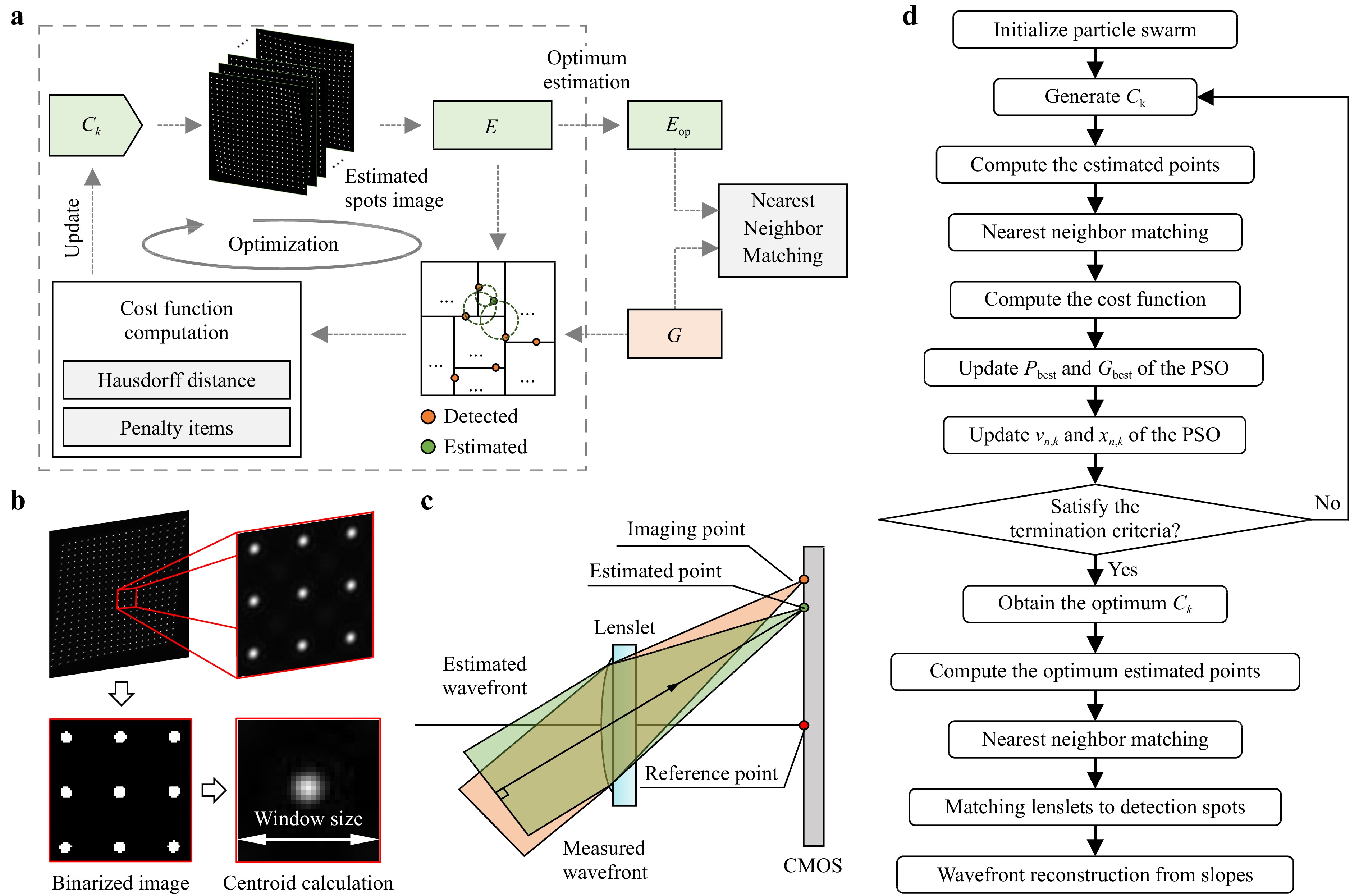
Fig. 1 Principle and schematic of ASM-SHWS. a Schematic of ASM-SHWS. b Segmentation and centroid extraction of spots from the original image. c Paraxial imaging model of SHWS. d Flowchart showing the implementation of ASM-SHWS using PSO.
The method for obtaining centroid coordinates from a spot image is illustrated in Fig. 1b. To account for the stark contrast in brightness between the spots and background, initial segmentation was conducted using Otsu’s method32. This was followed by identification of the connected components of the spots, which clarified the distribution of each individual spot. The centroid extraction process allows the determination of the set of detected points, G.
To search for the optimal incident wavefront corresponding to the detected spots, the ASM-SHWS requires a characterization that describes the distribution of the incident wavefront. One technique involves characterizing the incident wavefront with Zernike coefficients Ck (k = 1, 2, …, K, where K stands for the number of Zernike coefficients). With the SHWS paraxial imaging model (Fig. 1c), the positions of the spots aligned with each microlens can be calculated by
$$ \left\{\begin{array}{l} x_{e}^{(i)}=x_{r}^{(i)}+L \displaystyle\sum C_{k} \dfrac{\partial Z_{k}}{\partial x} \\ y_{e}^{(i)}=y_{r}^{(i)}+L \displaystyle\sum C_{k} \dfrac{\partial Z_{k}}{\partial y} \end{array}\right. $$ (1) Here, $ \left(x_{e}^{(i)}, y_{e}^{(i)}\right) $ denotes the centroid coordinates of the i-th spot (i = 1, 2, …, M, and M is the total count of microlens within the MLA); $ \left(x_{r}^{(i)}, y_{r}^{(i)}\right) $ represents the imaging position of the i-th microlens optical axis on the sensor, which is previously calibrated and considered as a reference position; Zk denotes the k-th Zernike polynomial term; and L denotes the distance between the MLA and sensor. To create the global matching cost function, the difference between the estimated and detected positions of the spots is initially calculated. To obtain a set of estimated points $ E=\left\{\left(x_{e}^{(1)}, y_{e}^{(1)}\right),\left(x_{e}^{(2)}, y_{e}^{(2)}\right) \ldots,\left(x_{e}^{(M)}, y_{e}^{(M)}\right)\right\} $, the centroid coordinate of all spots is computed. Next, the Hausdorff distance dH is calculated between sets E and G by
$$ \left\{\begin{array}{l} d_{\mathrm{FH}}(\boldsymbol{E}, \boldsymbol{G})=\sup _{e \in \boldsymbol{E}} \inf _{\boldsymbol{g} \in \boldsymbol{G}} d(e, g) \\ d_{\mathrm{BH}}(\boldsymbol{E}, \boldsymbol{G})=\sup _{g \in {\boldsymbol G} \in {\boldsymbol E}} \inf _{e \in \boldsymbol{E}} d(e, g) \\ d_{\mathrm{H}}=\max \left\{d_{\mathrm{FH}}, d_{\mathrm{BH}}\right\} \end{array}\right. $$ (2) Here, dFH and dBH denote the forward and backward Hausdorff distances, respectively; sup and inf denote the supremum and infimum, respectively; and $ d(\cdot) $ quantifies the distance from a point $ e \in \boldsymbol{E} $ to another $ g \in \boldsymbol{G} $. When calculating dH, it is necessary to establish point-to-point correspondences within sets E and G, using the nearest-neighbor principle. Consequently, two K-dimensional (K-D) trees were created based on the two-dimensional distribution of these points. The points associated with nodes within the corresponding K-D trees are selected as neighboring points, effectively reducing the temporal complexity. A penalty term was included in the cost function to maintain the accuracy of optimization direction. This safeguards against a single point serving as the nearest neighbor for multiple points.
Fig. 1d depicts the employment of Particle Swarm Optimization (PSO) for optimizing the incident wavefront via the Zernike coefficients Ck. PSO emulates bird flocking behavior through particle representations to obtain an optimal solution33. This is achieved by the particle adaptation of position and velocity based on population and individual experience, facilitating the estimation of the incident wavefront. Unlike gradient-based methods, PSO does not require gradient information related to the cost function and possesses strong global search capability, thereby avoiding localized optimization traps. Assuming a swarm size of N, the initial positions xn(0) (n = 1, 2, …, N) and initial velocities vn(0) are assigned to the N particles, where xn and vn are K-dimensional vectors. Throughout each iteration, it is necessary to compute the cost function for every particle to update the positions and velocities of the particle swarm.
$$ \left\{\begin{aligned} &\begin{aligned}v_{n, k}(t+1)=&w v_{n, k}(t)+c_{1} r_{1}\left[P_{b e s t}-x_{n, k}(t)\right]+\\& c_{2} F_{2}\left[G_{b \text { bess }}-x_{n, k}(t)\right] \end{aligned}\\ &x_{n, k}(t+1)=x_{n, k}(t)+v_{n, k}(t+1) \end{aligned}\right. $$ (3) Here, $ x_{n, k}(t) $ and $ v_{n, k}(t) $ represent the values of the k-th dimension of xn and vn after t iterations. The inertia weight (w) controls the effect of the previous velocity on the current velocity. The cognitive coefficient (c1) and social coefficient (c2) determine the influence of the best-known positions of the particle (Pbest) and swarm (Gbest). Generally, the inertia weight w is selected empirically within the range of 0–1, whereas the coefficients c1 and c2 are set within the range of 0–4. These coefficients were then multiplied by random numbers (0 < r1 < 1 and 0 < r2 < 1) to introduce stochasticity.
Using PSO, it is possible to attain the optimal estimation of Ck, which consequently makes it feasible to calculate the points within the estimated point set E. By establishing the correspondence between each point in set E and the microlenses, the correspondence between spots and microlenses can be deduced. Consequently, the slopes can be computed, and the incident wavefront can be reconstructed using a wavefront reconstruction algorithm such as modal decomposition or an iterative local reconstruction algorithm.
-
A thorough numerical simulation was performed to assess the effectiveness of the ASM-SHWS. The incident wavefront was generated by combining 15 Zernike polynomial terms and a random phase was produced by multiplying the Fourier spectrum of a random matrix by a two-dimensional Gaussian function34. The phase transfer function of the MLA was obtained using the thin-lens approximation. Subsequently, an SHWS model was developed using physical optics propagation, as described in our previous study35. The model utilized the angular spectrum theory to imitate the propagation of the incident wavefront from the MLA to the sensor. The numerical simulation adopted various parameters including a wavelength of 632.8 nm, an assembly distance of 5.2 mm between the MLA and sensor, a microlens pitch of 150 µm, a lens radius of curvature of 2.54 mm, a 19×19 MLA, and a pixel size of 5 µm.
Fig. 2 shows the simulation results. It displays the phase distribution of the incident wavefront with a peak-to-valley (PV) value of 2617 rad. Fig. 2a, b show the corresponding spot image formed on the sensor. The most notable spot deviation was observed in the bottom-right corner, which exhibited horizontal and vertical displacements of 249.1 and 263.4 pixels, respectively. By contrast, under the same simulation parameters, the conventional SHWS could only achieve a maximum limit of 15 pixels for the horizontal and vertical displacements. The measurable threshold of the conventional SHWS for local slopes of the simulated incident wavefront was surpassed by a factor of 24.17. The convergence curve of the optimization cost function is shown in Fig. 2c. In our numerical simulations and subsequent experiments, we implemented the widely used default values of the coefficients c1 = c2 = 1.49 and inertia weight w = 0.536. The swarm size was set to 100, and an initial search was performed for the first 15 Zernike polynomial coefficients. To begin the search, we initialized the Zernike coefficients to zero. Since the SHWS generally measures the low-frequency components of the incident wavefront, we designated appropriate upper and lower bounds for the 15 Zernike coefficients, with the bounds for higher-order terms being notably smaller than those for lower-order terms. Specifically, we set the bounds of the C1 to C6 terms as [−1, 1], C7 to C10 as [−0.1, 0.1], and C11 to C15 terms as [−0.01, 0.01], with the coordinate units in millimeters. The termination criterion was set as the absence of duplicate matching points and a Hausdorff distance below 6 pixels. The efficacy of this criterion in establishing accurate matching relationships has been demonstrated through various tests. The dynamic spot matching process is depicted in Movie S1, and the final spot-matching result are shown in Fig. 2d. Fig. 2e shows the relative reconstruction error (RE) of the wavefront reconstructed using a modal wavefront reconstruction algorithm employing Zernike polynomials37. The distribution of the relative RE was indicated by $ \mathrm{RE}=\left(W_{r}-W_{g}\right) / \mathrm{PV} $, where $ W_{r} $ and $ W_{g} $ represent the reconstructed and simulated incident wavefronts, respectively. The mean RE was 0.16% (Fig. 2e). The wavefront reconstruction procedure involved determining the slopes of the individual subwavefronts based on a paraxial approximation. An elevation in the paraxial approximation and a centroid positioning error occurred with significant spot deviations. As a result, the RE increased owing to the steep slope of the edge subwavefront. To confirm the robustness of the ASM-SHWS, the procedure was replicated to generate and evaluate 100 sets of high dynamic range incident wavefronts. All 100 wavefronts displayed mean RE values below 0.20% (Fig. 2f). Therefore, the ASM-SHWS demonstrated its capability to achieve large dynamic range wavefront reconstruction with remarkable robustness.
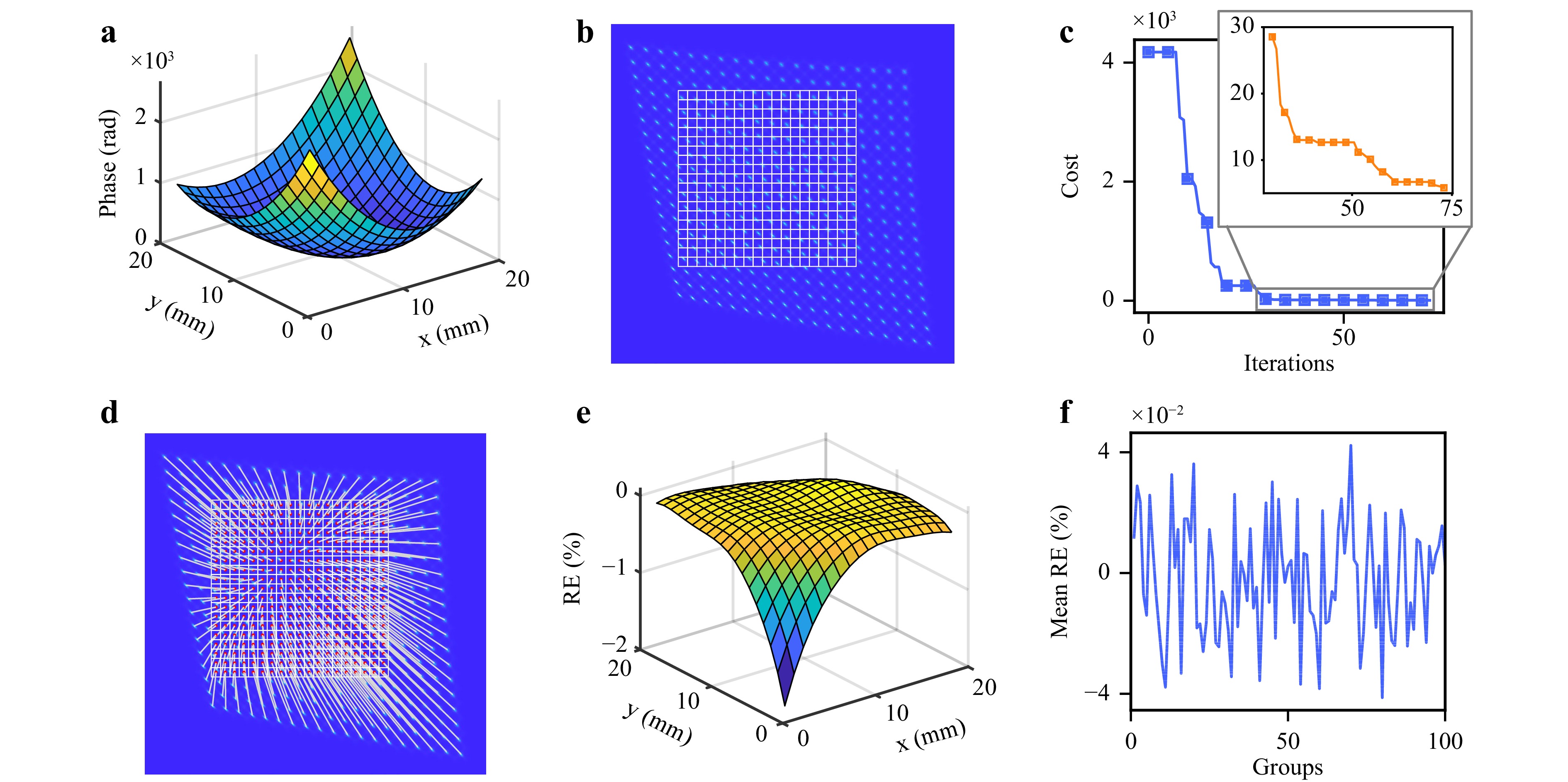
Fig. 2 Numerical simulation results. a Phase distribution of the incident wavefront. b The spot image where the white grids correspond to the microlens regions. c Convergence curve of the cost function during the optimization process. The upper right corner shows the iteration result where the cost is less than 30. d Spot matching result, where the spots are connected to their corresponding microlens by white lines. e Relative error of the incident wavefront. f Mean RE of the incident wavefront in 100 replicated simulations.
To comprehensively evaluate the performance of the ASM-SHWS, we conducted numerical simulations to investigate various types of large dynamic range wavefronts by manipulating distinct Zernike terms, such as oblique astigmatism (z3), defocus (z4), vertical trefoil (z6), and horizontal coma (z8). We assessed the maximum measurable dynamic range of ASM-SHWS for these diverse wavefronts and the corresponding PV values for these wavefronts were 3.95 × 10³, 3.49 × 10³, 1.10 × 10³, and 1.22 × 10³ rad (Fig. 3a). Different factors can influence the measurement performance of the ASM-SHWS across various wavefronts. This is primarily limited by the receiving area of the image sensor for wavefronts generated by manipulating the defocus (z4), whereas for other wavefronts, it is restricted by the resolution of the sensor relative to adjacent spots. A comparison was conducted to determine the maximum dynamic range attainable by the ASM-SHWS and conventional SHWS for distinct wavefronts. Fig. 3b shows the maximum PV and root mean square (RMS) results. The results illustrated that the dynamic range of ASM-SHWS in terms of the PV and RMS exceeded that of the conventional SHWS by 16.21 times.
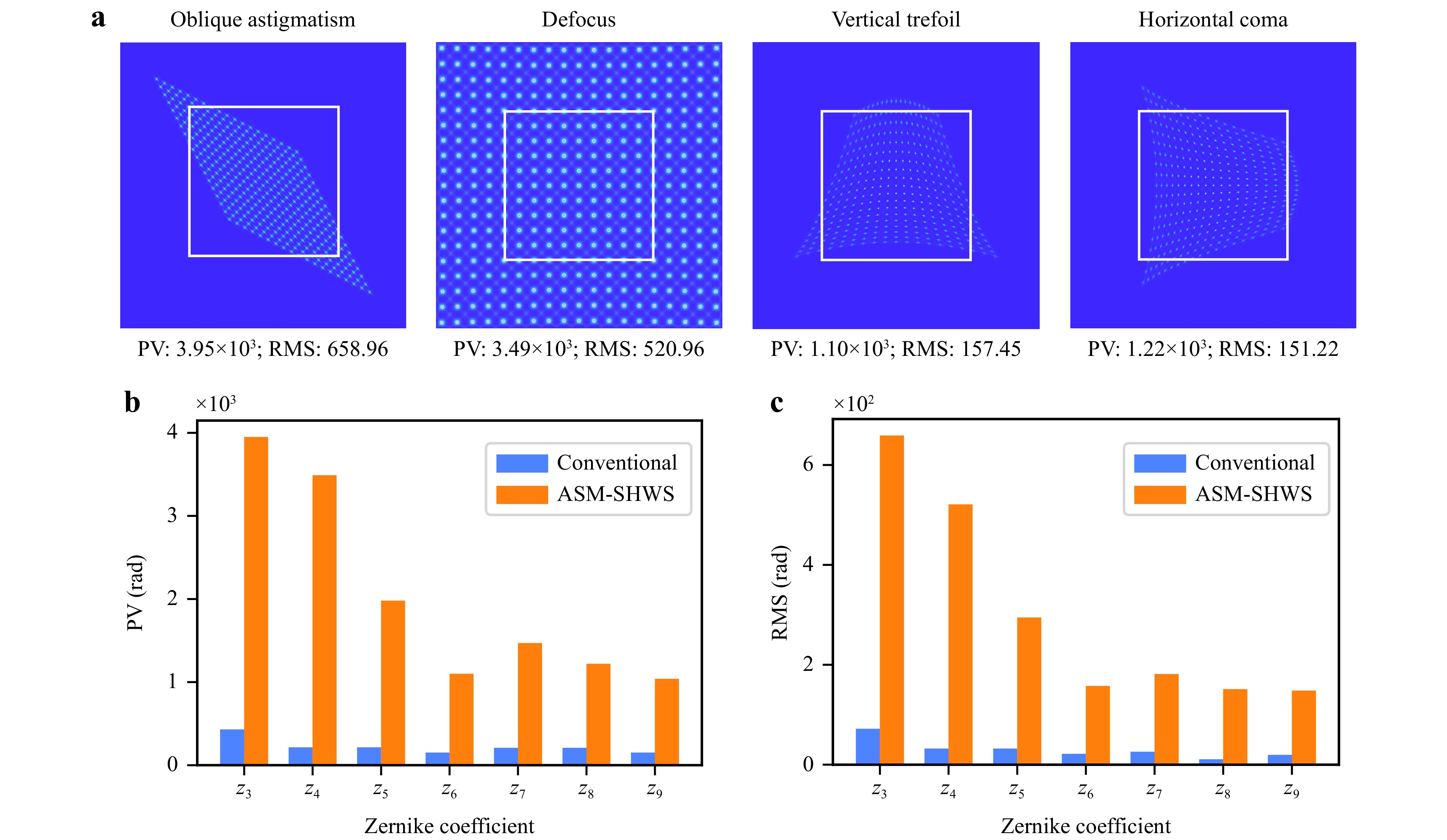
Fig. 3 Numerical comparison of ASM-SHWS and conventional SHWS for large dynamic range wavefront measurement. a Spot images for different types of large dynamic range wavefronts by manipulating different Zernike terms, including oblique astigmatism (z3), defocus (z4), vertical trefoil (z6) and horizontal coma (z8). The white boxes represent the border of the MLA. b The maximum PV and RMS of the measurable wavefronts in terms of Zernike terms.
In an SHWS, a unique wavefront corresponds to a unique distribution of focal spots; conversely, a unique distribution of focal spots can be inversely mapped to a unique wavefront. Even when some focal spots were missing, the remaining spots retained some wavefront characteristics. On this basis, the ASM-SHWS is designed to search for the optimal incident wavefront that best matches the distribution of the detected spots rather than a specific positional relationship between the detected spots. As a result, the ASM-SHWS shows global matching capability in reconstructing wavefronts with a large dynamic range even in cases where partial spot images are obtained owing to factors such as occlusion, illumination fluctuations, or limited imaging areas. Fig. 4a shows the spot-matching results with no missing spots. By manually inspecting the spot positions, we confirmed the accurate alignment of the spots and microlenses in Fig. 4a, and used it as a reference to assess the matching accuracy when certain spots were missing. We simulated spot images with different degrees of missing spots, including 13% missing spots at the periphery, 17% missing spots at the center, and 10%, 30%, and 50% missing spots within random regions. As shown in Fig. 4b-f, under different missing spots scenarios, the ASM-SHWS consistently and accurately matched the remaining spots to their respective microlenses, maintaining the consistency of the reference matching relationship shown in Fig. 4a. Thus, ASM-SHWS shows great robustness to both localized and random instances of missing spots.
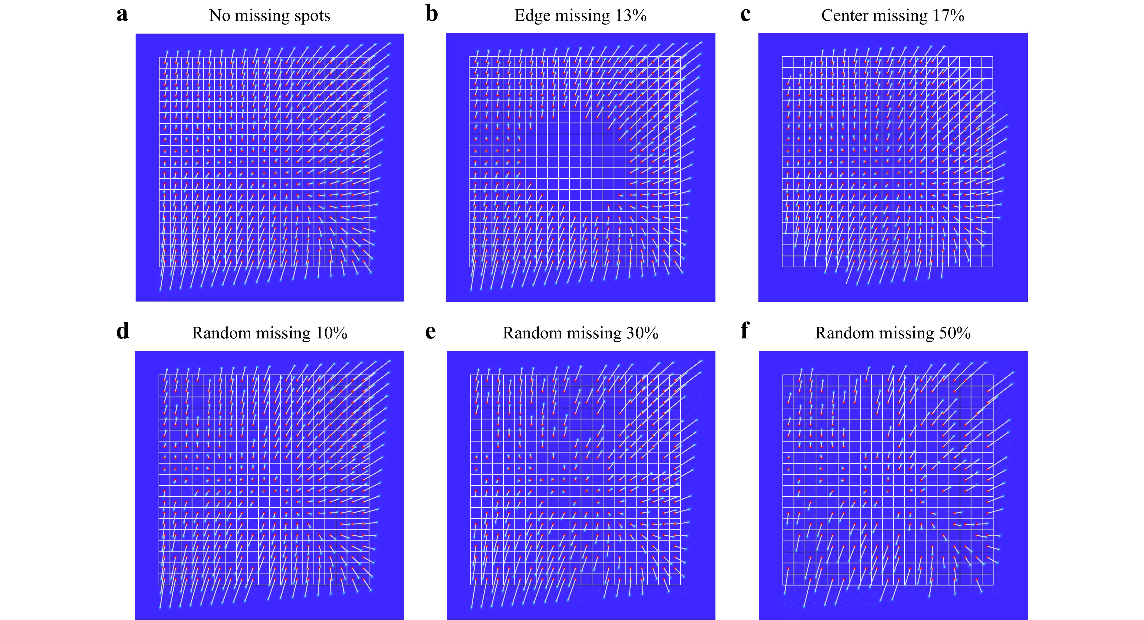
Fig. 4 Spots matching the results of ASM-SHWS with different degrees of missing spots: no missing spots a, missing 13% at the edge b, 17% at the center c and 10% d, 30% e and 50% f in the random region. The spots are connected to the corresponding microlens by white lines.
-
To validate the practical accuracy of the ASM-SHWS, we constructed an SHWS sensor using an MLA (MLA150-7AR, Thorlabs, Inc.) and a CMOS sensor (IMX249, Sony, Corp.). The SHWS was characterized by a pixel size of 5.86 µm and a microlens pitch of 150 µm. The distance between the MLA and the CMOS sensor, calibrated using the spherical wavefront calibration method38, was 5.42 mm. Given these parameters, the conventional SHWS demonstrated the ability to detect a maximum displacement of a single spot at 12.8 pixels, correlating to a maximum local slope of 13.84 mrad. The wavefront measurement setup is shown in Fig. 5a. The spherical wave emitted from the optical fiber was collimated and converged using a lens with a focal length of 100 mm. The SHWS was positioned both anterior and posterior to the focal point of the lens, allowing for the capture of highly curved converging and diverging spherical waves. The left sides of Fig. 5b, c show the spot images acquired at these positions. We reconstructed spherical waves using the ASM-SHWS and Zernike modal wavefront reconstruction algorithms. The reconstructed results after 41 and 47 iterations are shown on the right sides of Fig. 5b, c, respectively. Within our computing environment (MATLAB 2021a, CPU i7-10700), the computation time for the ASM-SHWS was 0.36 s and 0.41 s, respectively, which translates to ~8.8 ms per iteration. Subsequently, a spherical fitting procedure was performed on the reconstructed wavefronts, and their evaluation was quantified in terms of the Mean Relative Fitting Error (MRFE).
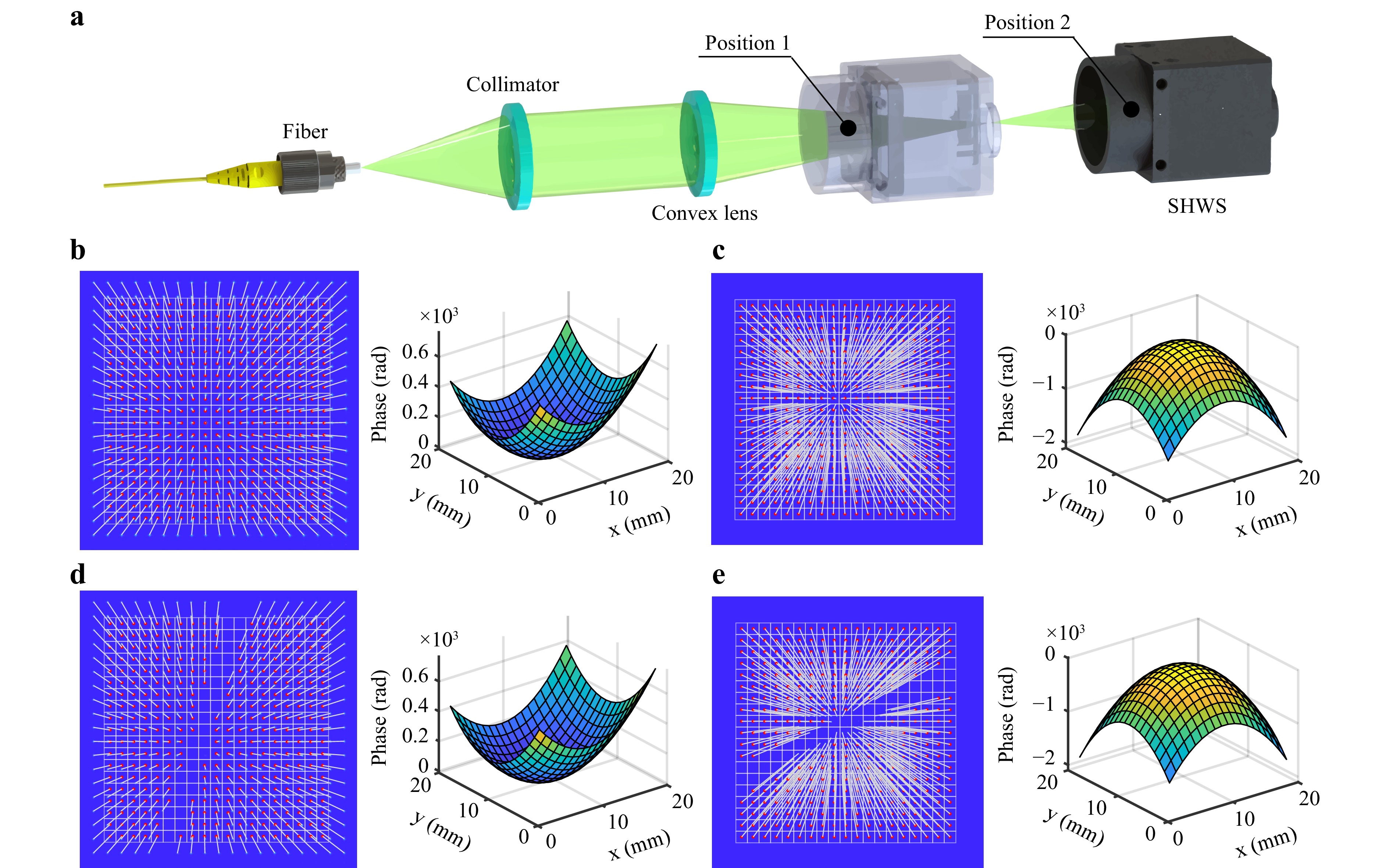
Fig. 5 Experimental results of wavefront measurement. a Experimental setup for the measurement of large curvature spherical waves using SHWS. b,c Spot matching and reconstruction results of ASM-SHWS for large curvature diverging b and converging c spherical waves. d,e Spot matching and reconstruction results of ASM-SHWS for large curvature diverging d and converging e spherical waves in the presence of missing spots.
$$ \operatorname{MRFE}=\frac{1}{N} \sum_{n=1}^{N} \frac{\left|W_{n}-S_{n}\right|}{\mathrm{PV}} $$ (4) Here, Wn and Sn denote the phase values of the n-th (n = 1, 2, 3, …, N) reconstruction point and the fitted sphere point, respectively. The MRFE values corresponding to the reconstructed diverging and converging spherical waves were 0.104% and 0.063%, respectively, compared with the fitted sphere (Fig. 5b, c). Notably, for the reconstructed diverging spherical wave, the farthest matched spot exhibited displacements of 47.50 and 47.76 pixels along the x and y directions, respectively. It manifested a local slope of 72.83 mrad, exceeding the conventional SHWS limit by a factor of 5.26 (Fig. 5b). Similarly, for the converging spherical wave, the farthest displacements in the x and y directions were 131.48 and 136.59 pixels, respectively, along a local slope of 204.98 mrad, exceeding those of the conventional SHWS by a factor of 14.81 (Fig. 5c).
Finally, we experimentally tested the measurement capability of the ASM-SHWS in the presence of missing spots. To induce missing spots in the image, we partially occluded the effective aperture, resulting in the configuration shown on the left sides of Fig. 5d, e. To counteract the centroid calculation errors caused by partially occluded spots, we implemented a threshold during image segmentation that ensured that only spots with sizes exceeding the threshold were considered for matching and subsequent reconstruction calculations. Consequently, the ASM-SHWS achieved accurate spot matching for the remaining spots in the scenarios with 32 missing spots (8.9%) and 45 missing spots (12.5%). Under these conditions, the MRFE values associated with the reconstructed diverging and converging spherical waves were 0.010% and 0.048%, respectively, compared with the fitted sphere (Fig. 5d, e). With 8.9% missing spots, the farthest matched spot in the reconstructed diverging spherical wave had a displacement of 47.56 and 47.82 pixels along the x and y directions, respectively. It also had a local slope of 72.91 mrad, exceeding the conventional SHWS limit by a factor of 5.27 (Fig. 5d). Similarly, for the converging spherical wave and with 12.5% missing spots, the farthest displacement in the x and y directions was 131.43 and 136.62 pixels, respectively. This was accompanied by a local slope of 204.97 mrad, which exceeds the conventional SHWS limit by a factor of 14.81 (Fig. 5e).
-
In this study, we presented the ASM-SHWS as a solution for large dynamic range wavefront measurements. By using an optimizer to establish global spot-to-microlens correspondences, the ASM-SHWS effectively overcomes the limitations inherent in conventional SHWS, which limit the measurement of maximum spot displacements within a single microlens. To quantify the deviation between the spot positions extracted from the estimated wavefront and actual detected spot positions, the Hausdorff distance was used to formulate the optimization cost function. For wavefront continuity and dimensionality reduction during optimization, Zernike coefficients were used as optimization parameters, and the PSO algorithm was used for a fast global search to determine the incident wavefront that best matches the detected spot positions. Additionally, a penalty term for repeated matching was introduced into the cost function to ensure an accurate optimization direction. Through numerical simulations, we demonstrated that the ASM-SHWS achieves a maximum measurable local slope that exceeds that of the conventional SHWS by a factor of 24.17. Furthermore, ASM-SHWS was shown to be effective in accurately matching spots, even when up to 50% of the spots were missing. The experiments showed that the ASM-SHWS can measure a spherical wave with a local slope of 204.97 mrad, achieving a 14.81-fold improvement over the conventional SHWS limit, even with 12.5% missing spots.
The ability of the ASM-SHWS to measure large dynamic range wavefronts can be improved further. Current limitations in dynamic range measurement arise primarily from scenarios where the wavefront slope is too steep, resulting in spots that exceed the sensor’s imaging range, and from cases where adjacent spots overlap, making it difficult to obtain accurate centroid coordinates during image segmentation. The former can be mitigated by enlarging the image sensor area, whereas the latter requires the application of more complex image segmentation algorithms. Furthermore, the ASM-SHWS is not limited to using Zernike polynomial coefficients to characterize the wavefront. Legendre polynomials and sub-wavefront slope values can also be used to further enhance the performance of the ASM-SHWS. The effectiveness of the ASM-SHWS is theoretically assured, provided that the measured wavefront maintains the necessary continuity and smoothness for the search of Zernike polynomial terms, along with accurate centroid extraction from the spot image. Moreover, on our current platform (MATLAB 2021a, CPU i7-10700), the algorithm achieves a processing speed of ~8.8 ms per iteration for a 19 × 19 array, typically converging within 100 iterations, resulting in a total runtime of less than 1 s. For a K-D tree, the time complexity of querying one point is O(log n), and when repeatedly searching for N points, the time complexity becomes O(nlog n). Fortunately, the cost of PSO generally reaches a 90% reduction after approximately 25 iterations, with the estimated spots being very close to the detected spots. This proximity is sufficient for matching spots with microlenses using a nearest neighbor algorithm, and significantly reduces the measurement time for ASM-SHWS when the number of iterations is reduced to 25. Additionally, the implementation of advanced nearest neighbor matching algorithms, iterative optimization algorithms, parallel computing architectures, and efficient programming languages promises the realization of a large dynamic range and real-time SHWS.
The proposed ASM-SHWS offers substantial potential for improving the capabilities of SHWS in detecting complex wavefronts. Conventional SHWS often faces a trade-off between the dynamic range and resolution, that is, reducing the microlens pitch to increase resolution can lead to a reduction in the dynamic range. By contrast, the ASM-SHWS overcomes the limitation of the microlens pitch to the maximum measurable local slope. This advancement enables the measurement of complex wavefronts characterized by both a large dynamic range and high resolution. Furthermore, the ASM-SHWS excels at measuring wavefronts even with missing spots. This demonstrates its ability to handle complex measurement conditions. By effectively mitigating the disadvantages of resolution and dynamic range, the ASM-SHWS method expands the application scope of the SHWS, thus promoting progress in fields such as astronomical exploration and industrial inspection.
-
Open Access This article is licensed under a Creative Commons Attribution 4.0 International License, which permits use, sharing, adaptation, distribution and reproduction in any medium or format, as long as you give appropriate credit to the original author(s) and the source, provide a link to the Creative Commons license, and indicate if changes were made. The images or other third party material in this article are included in the article′s Creative Commons license, unless indicated otherwise in a credit line to the material. If material is not included in the article′s Creative Commons license and your intended use is not permitted by statutory regulation or exceeds the permitted use, you will need to obtain permission directly from the copyright holder. To view a copy of this license, visit http://creativecommons.org/licenses/by/4.0/.
-
This work was supported by the Fundamental Research Funds for the Central Universities of Shanghai Jiao Tong University and the Shanghai Jiao Tong University 2030 Initiative (No. WH510363001-10), and the Oceanic Interdisciplinary Program of Shanghai Jiao Tong University (No. SL2022ZD205), the Science Foundation of the Donghai Laboratory (No. DH-2022KF01001), and National Natural Science Foundation of China (No. 62205189).
Large dynamic range Shack-Hartmann wavefront sensor based on adaptive spot matching
- Light: Advanced Manufacturing , Article number: (2024)
- Received: 16 September 2023
- Revised: 29 December 2023
- Accepted: 08 January 2024 Published online: 16 March 2024
doi: https://doi.org/10.37188/lam.2024.007
Abstract: The Shack-Hartmann wavefront sensor (SHWS) is widely used for high-speed, precise, and stable wavefront measurements. However, conventional SHWSs encounter a limitation in that the focused spot from each microlens is restricted to a single microlens, leading to a limited dynamic range. Herein, we propose an adaptive spot matching (ASM)-based SHWS to extend the dynamic range. This approach involves seeking an incident wavefront that best matches the detected spot distribution by employing a Hausdorff-distance-based nearest-distance matching strategy. The ASM-SHWS enables comprehensive spot matching across the entire imaging plane without requiring initial spot correspondences. Furthermore, due to its global matching capability, ASM-SHWS can maintain its capacity even if a portion of the spots are missing. Experiments showed that the ASM-SHWS could measure a high-curvature spherical wavefront with a local slope of 204.97 mrad, despite a 12.5% absence of spots. This value exceeds that of the conventional SHWS by a factor of 14.81.
Research Summary
Adaptive spot matching empowers Shack-Hartmann sensors for high-curvature wavefront measurements
Traditional Shack-Hartmann sensors face a limitation that the focused spot from each microlens is restricted to a single microlens, resulting in a limited dynamic range. Qiao-Zhi He from China’s Shanghai Jiao Tong University and colleagues report a development that extends the dynamic range of the Shack-Hartmann wavefront sensor by an order of magnitude without increasing system complexity shows promise. Their approach introduces an adaptive spot matching method, utilizing a nearest-distance matching strategy to identify the incident wavefront that best matches the detected spot distribution. This method can achieve comprehensive spot matching across the entire imaging plane without requiring initial spot correspondences, even when some spots are missing. The team demonstrated measuring a high-curvature spherical wavefront with a high slope of 204.97 mrad despite a 12.5% absence of spots, exceeding the capability of traditional Shack-Hartmann sensors by a factor of 14.81.
Rights and permissions
Open Access This article is licensed under a Creative Commons Attribution 4.0 International License, which permits use, sharing, adaptation, distribution and reproduction in any medium or format, as long as you give appropriate credit to the original author(s) and the source, provide a link to the Creative Commons license, and indicate if changes were made. The images or other third party material in this article are included in the article′s Creative Commons license, unless indicated otherwise in a credit line to the material. If material is not included in the article′s Creative Commons license and your intended use is not permitted by statutory regulation or exceeds the permitted use, you will need to obtain permission directly from the copyright holder. To view a copy of this license, visit http://creativecommons.org/licenses/by/4.0/.

 DownLoad: